Uncertainty-Aware and Reliable Neural MIMO
Receivers via Modular Bayesian Deep Learning
Tomer Raviv, Sangwoo Park, Osvaldo Simeone, and Nir Shlezinger
Abstract—Deep learning is envisioned to play a key role in
the design of future wireless receivers. A popular approach
to design learning-aided receivers combines deep neural net-
works (DNNs) with traditional model-based receiver algorithms,
realizing hybrid model-based data-driven architectures. Such
architectures typically include multiple modules, each carrying
out a different functionality dictated by the model-based receiver
workflow. Conventionally trained DNN-based modules are known
to produce poorly calibrated, typically overconfident, decisions.
Consequently, incorrect decisions may propagate through the ar-
chitecture without any indication of their insufficient accuracy. To
address this problem, we present a novel combination of Bayesian
deep learning with hybrid model-based data-driven architectures
for wireless receiver design. The proposed methodology, referred
to as modular Bayesian deep learning, is designed to yield
calibrated modules, which in turn improves both accuracy and
calibration of the overall receiver. We specialize this approach
for two fundamental tasks in multiple-input multiple-output
(MIMO) receivers – equalization and decoding. In the presence
of scarce data, the ability of modular Bayesian deep learning
to produce reliable uncertainty measures is consistently shown
to directly translate into improved performance of the overall
MIMO receiver chain.
I. INTRODUCTION
Deep neural networks (DNNs) were shown to successfully
learn complex tasks from data in domains such as computer
vision and natural language processing. This dramatic success
has led to a burgeoning interest in the design of DNN-
aided communications receivers [2]–[6]. While traditional re-
ceiver algorithms are based on the mathematical modelling of
signal transmission, propagation, and reception, DNN-based
receivers learn their mapping from data without relying on
such accurate modelling. Consequently, DNN-aided receivers
can operate efficiently in scenarios where the channel model
is unknown, highly complex, or difficult to optimize [7]. The
incorporation of deep learning into receiver processing is thus
often envisioned to be an important contributor to meeting the
rapidly increasing demands of wireless systems in throughput,
coverage, and robustness [8].
Parts of this work were presented at the 2023 IEEE International Conference
on Communications (ICC) as the paper [1]. T. Raviv and N. Shlezinger are
with the School of ECE, Ben-Gurion University of the Negev, Beer-Sheva,
Simeone are with King’s Communication Learning & Information Processing
(KCLIP) lab, Centre for Intelligent Information Processing Systems (CIIPS),
at the Department of Engineering, King’s College London, U.K. (email:
{sangwoo.park; osvaldo.simeone}@kcl.ac.uk). The work of T. Raviv and
N. Shlezinger was partially supported by the Israeli Innovation Authority.
The work of O. Simeone was partially supported by the European Union’s
Horizon Europe project CENTRIC (101096379), by an Open Fellowship of
the EPSRC (EP/W024101/1), by the EPSRC project (EP/X011852/1), and
by Project REASON, a UK Government funded project under the Future
Open Networks Research Challenge (FONRC) sponsored by the Department
of Science Innovation and Technology (DSIT).
Despite their promise in facilitating physical layer com-
munications, particularly or multiple-input multiple-output
(MIMO) systems, the deployment of DNNs faces several
challenges that may limit their direct applicability to wireless
receivers. The dynamic nature of wireless channels combined
with the limited computational and memory resources of wire-
less devices indicates that MIMO receiver processing is fun-
damentally distinct from conventional deep learning domains,
such as computer vision and natural language processing [9],
[10]. Specifically, the necessity for online training may arise
due to the time-varying settings of wireless communications.
Nonetheless, pilot data corresponding to new channels is
usually scarce. DNNs trained using conventional deep learn-
ing mechanisms, i.e., via frequentist learning, are prone to
overfitting in such settings [11]. Moreover, they are likely to
yield poorly calibrated outputs [12], [13], e.g., produce wrong
decisions with high confidence.
A candidate approach to design DNN-aided receivers that
can be trained with limited data incorporates model-based
receiver algorithms as a form of inductive bias into a hy-
brid model-based data-driven architecture [14]–[16]. One
such model-based deep learning methodology is deep unfold-
ing [17]. Deep unfolding converts an iterative optimizer into a
discriminative machine learning system by introducing train-
able parameters within each of a fixed number of iterations
[16], [18]. Deep unfolded architectures treat each iteration
as a trainable module, obtaining a modular and interpretable
DNN architecture [19], with each module carrying out a
specific functionality within a conventional receiver processing
algorithm. Modularity is informed by domain knowledge,
potentially enhancing the generalization capability of DNN-
based receivers [20]–[25].
Hybrid model-based data-driven methods require less data
to reliably train compared to black box architectures. Yet, the
resulting system may be negatively affected by the inclusion
of conventionally trained DNN-based modules, i.e., DNNs
trained via frequentist learning [13]. This follows from the
frequent overconfident decisions that are often produced by
such conventional DNNs, particularly when learning from
limited data sets. Such poorly calibrated DNN-based modules
may propagate inaccurate predictions through the architecture
without any indication of their insufficient accuracy.
The machine learning framework of Bayesian learning
accommodates learning techniques with improved calibra-
tion compared with frequentist learning [13], [26]–[28]. In
Bayesian deep learning, the parameters of a DNN are treated
as random variables. Doing so provides means to quantify
the epistemic uncertainty, which arises due to lack of training
data. Bayesian deep learning was shown to improve the
reliability of DNNs in wireless communication systems [29],
1
arXiv:2302.02436v3 [cs.IT] 14 Mar 2024
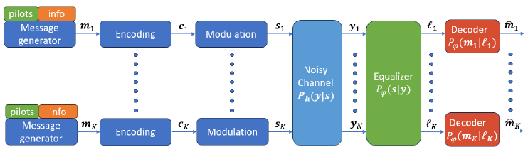
Fig. 1: The communication system studied in this paper.
[30]. Nonetheless, these existing studies adopt black-box DNN
architectures. Thus, the existing approaches do not leverage
the modularity of model-based data-driven receivers, and do
not account for the ability to assign interpretable meaning to
intermediate features exchanged in model-based deep learning
architectures.
In this work we present a novel methodology, referred to
as modular Bayesian deep learning, that combines Bayesian
learning with hybrid model-based data-driven architectures for
DNN-aided receivers. The proposed approach calibrates the
internal DNN-based modules, rather than merely calibrating
the overall system output. This has the advantage of yielding
well-calibrated soft outputs that can benefit downstream tasks,
as we empirically demonstrate.
Our main contributions are summarized as follows.
• Modular Bayesian deep learning: We introduce a mod-
ular Bayesian deep learning framework that integrates
Bayesian learning with model-based deep learning. Ac-
counting for the modular architecture of hybrid model-
based data-driven receivers, Bayesian learning is applied
on a per-module basis, enhancing the calibration of soft
estimates exchanged between internal DNN modules.
The training procedure is based on dedicated sequential
Bayesian learning operation, which boosts calibration of
internal modules while encouraging subsequent modules
to exploit these calibrated features.
• Modular Bayesian deep MIMO receivers: We special-
ize the proposed methodology to MIMO receivers. To this
end, we adopt two established DNN-aided architectures
– the DeepSIC MIMO equalizer of [21] and the deep
unfolded weighted belief propagation (WBP) soft decoder
of [31] – and derive their design as modular Bayesian
deep learning systems.
• Extensive experimentation: We evaluate the advantages
of modular Bayesian learning for deep MIMO receivers
based on DeepSIC and WBP. Our evaluation first con-
siders equalization and decoding separately, followed by
an evaluation of the overall receiver chain composed of
the cascade of equalization and decoding. The proposed
Bayesian modular approach is systematically shown to
outperform conventional frequentist learning, as well as
traditional Bayesian black-box learning, while being re-
liable and interpretable,
The remainder of this paper is organized as follows: Sec-
tion II formulates the considered MIMO system model, and re-
views some necessary preliminaries on Bayesian learning and
model-based deep receivers. Section III presents the proposed
methodology of modular Bayesian learning, and specializes it
for MIMO equalization using DeepSIC and for decoding using
the WBP. Our extensive numerical experiments are reported
in Section IV, while Section V provides concluding remarks.
Throughout the paper, we use boldface letters for multivari-
ate quantities, e.g., x is a vector; calligraphic letters, such as
X for sets, with |X | being the cardinality of X ; and R for the
set of real numbers. The notation (·)
T
stands for the transpose
operation.
II. SYSTEM MODEL AND PRELIMINARIES
In this section, we describe the MIMO communication
system under study in Subsection II-A, and review the con-
ventional frequentist learning of MIMO receivers in Subsec-
tion II-B. Then, we briefly present basics of model-based
learning for deep receivers in Subsection II-C, and review our
main running examples of DeepSIC [21] and WBP [31].
A. System Model
We consider an uplink MIMO digital communication system
with K single-antenna users. The users transmit encoded mes-
sages, independently of each other, to a base station equipped
with N antennas. Each user of index k uses a linear block
error-correction code to encode a length m binary message
m
k
∈ {0, 1}
m
. Encoding is carried out by multiplication with
a generator matrix G, resulting in a length C ≥ m codeword
given by c
k
= G
T
m
k
∈ {0, 1}
C
. The same codebook is em-
ployed for all users. The messages are modulated, such that
each symbol s
k
[i] at the ith time index is a member of the
set of constellation points S. The transmitted symbols vector
form the K × 1 vector s[i] = [s
1
[i] . . . s
K
[i]] ∈ S
K
.
We adopt a block-fading model, i.e., the channel remains
constant within a block of duration dictated by the coherence
time of the channel. A single block of duration T
tran
is
generally divided into two parts: the pilot part, composed of
T
pilot
pilots, and the message part of T
info
= T
tran
− T
pilot
information symbols. The corresponding indices for transmit-
ted pilot symbols and information symbols are written as
T
pilot
= {1, ..., T
pilot
}, and T
info
= {T
pilot
+ 1, ..., T
tran
},
respectively.
To accommodate complex and non-linear channel models,
we represent the channel input-output relationship by a generic
2

conditional distribution. Accordingly, the corresponding re-
ceived signal vector y[i] ∈ R
N
is determined as
y[i] ∼ P
h
(y[i]|s[i]), (1)
which is subject to the unknown conditional distribution
P
h
(·|·) that depends on the current channel parameters h.
The received channel outputs in (1) are processed by the
receiver, whose goal is to recover correctly each message.
This estimate of the kth user message is denoted by
ˆ
m
k
. This
mapping can be generally divided into two different tasks: (i)
equalization and (ii) decoding. Equalization maps the received
signal y[i] as an input into a vector of soft symbols estimates
for each user, denoted
ˆ
P
1
[i], . . . ,
ˆ
P
K
[i]. Decoding is done
for each user separately, obtaining an estimation
ˆ
m
k
of the
transmitted message from the soft probability vectors {
ˆ
P
k
[i]}
i
corresponding to the codeword. The latter often involves first
obtaining a soft estimate for each bit in the message, where
we use
ˆ
L
k
[v] to denote the estimated probability that the vth
bit in the kth message is one. The entire communication chain
is illustrated in Fig. 1.
B. Frequentist Deep Receivers
Deep receivers employ DNNs to map the block of channel
output into the transmitted message, i.e., as part of the equal-
ization and/or decoding operations. In conventional frequentist
learning, optimization of the parameter vector φ dictating the
receiver mappings is typically done by minimizing the cross-
entropy loss using a labelled pair of inputs and outputs [3],
i.e.,
φ
freq
= arg min
φ
L
CE
(φ). (2)
For example, to optimize an equalizer (formulated here for a
single user case for brevity), one employs T
pilot
pilot symbols
and their corresponding observed channel outputs to compute
L
CE
(φ) = −
1
|T
pilot
|
X
i∈T
pilot
log P
φ
(s[i]|y[i]). (3)
In (3), P
φ
(s[i]|y[i]) is the soft estimate associated with the
symbol s[i] computed from y[i] with a DNN-aided equalizer
with parameters φ. When such an equalizer is used, the
stacking of {P
φ
(s|y[i])}
s∈S
forms the soft estimate
ˆ
P [i].
Calibration is based on the reliability of its soft estimates.
In particular, a prediction model P
φ
(s[i]|y[i]) as in the above
DNN-aided equalizer example is perfectly calibrated if the
conditional distribution of the transmitted symbols given the
predictor’s output satisfies the equality [12]
P (s[i] =
ˆ
s[i]|P
φ
(
ˆ
s[i]|y[i]) = π) = π for all π ∈ [0, 1]. (4)
When (4) holds, then the soft outputs of the prediction model
coincide with the true underlying conditional distribution.
C. Hybrid Model-Based Data-Driven Architectures
As mentioned in Section I, two representative examples
of hybrid model-based data-driven architectures employed by
deep receivers are: (i) the DeepSIC equalizer of [21]; and
(ii) the unfolded WBP introduced in [31], [32] for channel
Algorithm 1: DeepSIC Inference
Input: Channel output y[i]; Parameter vector φ
SIC
.
Output: Soft estimations for all users {
ˆ
P
k
[i]}
K
k=1
.
1 DeepSIC Inference
2 Generate an initial guess {
ˆ
P
(k,0)
}
K
k=1
.
3 for q ∈ {1, ..., Q} do
4 for k ∈ {1, ..., K} do
5 Calculate
ˆ
P
(k,q)
by (5).
6 return {
ˆ
P
k
[i] =
ˆ
P
(k,Q)
}
K
k=1
decoding. As these architectures are employed as our main
running examples in the sequel, we next briefly recall their
formuation.
1) DeepSIC: The DeepSIC architecture proposed in [21]
is a modular model-based DNN-aided MIMO demodulator,
based on the classic soft interference cancellation (SIC) al-
gorithm [33]. SIC operates in Q iterations. This equalization
algorithm refines an estimate of the conditional probability
mass function for the constellation points in S denoted by
ˆ
P
(k,q)
, for each symbol transmitted by a user of index k,
throughout the iterations q = 1, . . . , Q. The estimate is
generated for every user k ∈ {1, . . . , K} and every iteration
q ∈ {1, . . . , Q} by using the soft estimates {
ˆ
P
(l,q−1)
}
l̸=k
of
the interfering symbols {s
l
[i]}
l̸=k
obtained in the previous
iteration q − 1 as well as the channel output y[i]. This
procedure is illustrated in Fig. 2(a).
In DeepSIC, interference cancellation and soft detection
steps are implemented with DNNs. Specifically, the soft esti-
mate of the symbol transmitted by kth user in the qth iteration
is calculated by a DNN-based classifying module with param-
eter vector φ
(k,q)
. Accordingly, the |S| × 1 probability mass
function vector for user k at iteration q under time index i can
be obtained as
ˆ
P
(k,q)
=
n
P
φ
(k,q)
(s|y[i], {
ˆ
P
(l,q−1)
[i]}
l̸=k
)
o
s∈S
, (5)
where DeepSIC is parameterized by the set of model parameter
vectors φ
SIC
= {{φ
(k,q)
}
K
k=1
}
Q
q=1
. The entire DeepSIC archi-
tecture is illustrated in Fig. 2(b) and its inference procedure
is summarized in Algorithm 1.
In the original formulation in [21], DeepSIC is trained in a
frequentist manner, i.e., by minimizing the cross-entropy loss
(3). By treating each user k = 1, . . . , K equally, the resulting
loss is given by
L
SIC
CE
(φ) =
K
X
k=1
L
MSIC
CE
(φ
(k,Q)
), (6)
where the user-wise cross-entropy is evaluated over the pilot
set T
pilot
as
L
MSIC
CE
(φ
(k,q)
) = −
1
|T
pilot
|
×
X
i∈T
pilot
log P
φ
(k,q)
(s
k
[i]|y[i], {
ˆ
P
(l,q−1)
[i]}
l̸=k
). (7)
In [21], the soft estimates for each user of index k were
obtained via the final soft output, i.e.,
ˆ
P
k
[i] is obtained as
3

Fig. 2: (a) Iterative SIC; and (b) DeepSIC [21]. In this paper,
we introduce modular Bayesian learning, which calibrates the
internal modules of the DeepSIC architecture with the double
goal of improving end-to-end accuracy and of producing well-
calibrated soft outputs for the benefit of downstream tasks.
ˆ
P
(k,Q)
. It was shown in [21] that under such setting, DeepSIC
can outperform frequentist black-box deep receivers under
limited pilots scenarios. However, its calibration performance
is not discussed.
2) Weighted Belief Propagation: Belief propagation (BP)
[34] is an efficient algorithm for calculating the marginal
probabilities of a set of random variables whose relationship
can be represented as a graph. A graphical representation used
in channel coding is the Tanner graph of linear error-correcting
codes [35]. A Tanner graph is a bipartite graph with two types
of nodes: variable nodes and check nodes. The variable nodes
correspond to bits of the encoded message, and the check
nodes represent constraints that the message must satisfy.
In the presence of loops in the graph, BP is generally
suboptimal. Its performance can be improved by weighting
the messages via a learnable variant of the standard BP, called
WBP [31], [32]. In WBP, the messages passed between nodes
in the graphical model are weighted based on the relative soft-
information they represent. These weights are learned from
data by unfolding the message passing iterations of BP into
a machine learning architecture. In particular, the message
passing algorithm operates by iteratively passing messages
over edges from variables nodes to check nodes and vice versa.
As the decoder is applied to each user seperately, we omit
the user index k in the following. To formulate the decoder,
let the WBP message from variable node v to check node h
at iteration q be denoted by M
(q )
v →h
, and from check node h
to variable node v by M
(q )
h→v
. The messages are initialized
M
(q )
v →h
= M
(q )
h→v
= 0 for all (v, h) ∈ H, where H denotes
all valid variable-check connections. For instance, validity is
determined for linear block codes by the element in the vth
row and hth column in the parity check matrix. The input log
likelihood ratio (LLR) values to the decoder are initialized
from the outputs of the detection phase.
Algorithm 2: WBP Inference
Input: LLR values ℓ; Parameter vector φ
WBP
.
Output: Soft estimations for message bits
ˆ
L.
1 WBP Inference
2 Initialize M
(0)
v →h
= M
(0)
h→v
= 0.
3 for q ∈ {1, ..., Q} do
4 for (v, h) ∈ H do
5 Update M
(q )
v →h
by (8).
6 for (v, h) ∈ H do
7 Update M
(q )
h→v
by (9).
8 Calculate
ˆ
L by (10) with q = Q.
9 return
ˆ
L
To this end, one first finds the soft estimate
˜
c ∈ R
C
of
the codeword c. Given the ith soft symbol probability
ˆ
P [i],
the soft estimate
˜
c can be found by translating
ˆ
P [i] to r =
log
2
|S| soft bits probabilities {
˜
c[i · r], ...,
˜
c[i · r + r − 1]} with
˜
c[v] = P (c[v] = 1|
ˆ
P [i]) for v = i · r, ..., i · r + r − 1. Then
the LLRs are computed by
ℓ[v] = log
˜
c[v]
1 −
˜
c[v]
,
and we use the vector ℓ to denote the stacking of ℓ[v] for all
bit indices v corresponding to a given codeword.
After initialization, the iterative algorithm begins. Variable-
to-check messages are updated according to the rule. i.e.,
M
(q )
v →h
= tanh
1
2
(ℓ[v] +
X
(v ,h
′
)∈H
h
′
̸=h
W
(q )
h
′
→v
M
(q −1)
h
′
→v
)
, (8)
with the parameters φ
(q )
= {W
(q )
}, where W
(q )
is a
weights’ matrix. The check-to-variable messages are updated
by a non-weighted rule
M
(q )
h→v
= 2 arctanh
Y
(v
′
,h)∈H
v
′
̸=v
M
(q )
v
′
→h
. (9)
The bit-wise probabilities are obtained from the messages via
ˆ
L
(q )
[v] = tanh
1
2
(ℓ[v] +
X
(v ,h
′
)∈H
W
(q )
h
′
→v
M
(q −1)
h
′
→v
)
(10)
The update rules are performed on every combination of
v, h for Q iterations. Finally, the codeword is estimated as
the hard-decision on the probability vector
ˆ
L, which is the
stacking of the bit-wise probabilities
ˆ
L
(Q)
[v] for every v in
the codeword. The entire inference procedure for a given
WBP paramterization φ
WBP
= {φ
(q )
}
Q
q=1
is summarized in
Algorithm 2.
The parameters of WBP, φ
WBP
, are learned from data.
Specifically, the decoder is trained to minimize the following
cross-entropy multi-loss (3) over the pilots set C
pilot
=
{1, . . . , r ∗ T
pilot
}
L
WBP
CE
(φ) =
Q
X
q =1
L
MWBP
CE
(φ
(q )
), (11)
4

Algorithm 3: Bayesian DeepSIC
Input: Channel output y[i]; Distribution over entire
architecture p
b
(φ
SIC
); Ensemble size J.
Output: Soft estimations for all users {
ˆ
P
k
[i]}
K
k=1
.
1 Bayesian Inference
2 for j ∈ {1, ..., J} do
3 Generate φ
SIC
j
∼ p
b
(φ
SIC
);
4 {
ˆ
P
k,j
[i]}
K
k=1
← DeepSIC (y[i], φ
SIC
j
);
5 return {
ˆ
P
k
[i] =
1
J
P
J
j=1
ˆ
P
k,j
[i]}
K
k=1
with the cross-entropy loss at iteration q defined as
L
MWBP
CE
(φ
(q )
) =
−
1
|C
pilot
|
X
v ∈C
pilot
log P
φ
(q)
(m[v]|ℓ[v], {M
(q −1)
h
′
→v
}). (12)
In (12), P
φ
(q)
(m[v]|ℓ[v], {M
(q −1)
h
′
→v
}) is the binary probability
vector computed for the vth bit of the message, i.e., m[v].
III. MODULAR BAYESIAN DEEP LEARNING
Bayesian learning is known to improve the calibration
of black-box DNNs models by preventing overfitting [29],
[36]. In this section, we fuse Bayesian learning with hybrid
model-based data-driven deep receivers. To this end, we first
present the direct application of Bayesian learning to deep
receivers in Subsection III-A, and illustrate the approach for
DeepSIC and WBP in Subsection III-B. Then, we introduce
the proposed modular Bayesian framework, and specialize it
again to DeepSIC and WBP in Subsection III-C. We conclude
with a discussion presented in Subsection III-D.
A. Bayesian Learning
Bayesian learning treats the parameter vector φ of a ma-
chine learning architecture as a random vector. This ran-
dom vector obeys a distribution p
b
(φ) that accounts for the
available data and for prior knowledge. Most commonly, the
distribution is obtained by minimizing the free energy loss,
also known as negative evidence lower bound (ELBO) [13],
via
p
b
(φ) = arg min
p
′
E
φ∼p
′
(φ)
[L
CE
(φ)]
+
1
β
KL(p
′
(φ)||p
prior
(φ))
. (13)
The Kullback-Leibler (KL) divergence term in (13), given by
KL
p
′
(φ)||p(φ)
≜ E
p
′
(φ)
h
log
p
′
(φ)
p(φ)
i
,
regularizes the optimization of p
b
(φ) with a prior distribution
p
prior
(φ). The hyperparameter β > 0, known as the inverse
temperature parameter, balances the regularization impact
[11], [13].
Algorithm 4: Bayesian WBP
Input: LLR values ℓ; Distribution over entire
architecture p
b
(φ
WBP
); Ensemble size J.
Output: Soft estimations for message bits
ˆ
L.
1 Bayesian Inference
2 for j ∈ {1, ..., J} do
3 Generate φ
WBP
j
∼ p
b
(φ
WBP
);
4
ˆ
L
j
← WBP (ℓ, φ
WBP
j
);
5 return
ˆ
L =
1
J
P
J
j=1
ˆ
L
j
Once optimization based on (13) is carried out, Bayesian
learning aims at having the output conditional distribution
approximate the stochastic expectation
P
p
b
= E
φ∼p
b
(φ)
[P
φ
]. (14)
The expected value in (14) is approximated by ensemble
decision, namely, combining multiple predictions, with each
decision based on a different realization of φ sampled from
the optimized distribution p
b
(φ). Bayesian prediction (14)
can account for the epistemic uncertainty residing in the
optimal model parameters. This way, it can generally obtain
a better calibration performance as compared to frequentist
learning [29], [30].
B. Conventional Bayesian Learning for Deep Receivers
The conventional application of Bayesian learning includes
obtaining the distribution over the set of model parameters
vectors p
b
(φ). Afterwards, one can proceed to inference,
where an ensembling over multiple realizations of parameters
vectors, drawn from p
b
(φ), leads to more reliable estimate.
Below, we specialize this case for our main running examples
of deep receiver architectures: DeepSIC and WBP.
1) DeepSIC: The DeepSIC equalizer is formulated in Al-
gorithm 1 for a deterministic (frequentist) parameter vector.
When conventional Bayesian learning is employed, one ob-
tains a distribution p
b
(φ
SIC
) over the set of model parameter
vectors φ
SIC
by minimizing the free energy loss (13). Using
these distribution, the prediction for information symbols is
computed as
P
p
b
(s
k
[i]|y[i]) = E
φ
SIC
∼p
b
(φ
SIC
)
P
φ
SIC
(s
k
[i]|y[i])
, (15)
for each data symbol at i ∈ T
info
, with soft prediction
ˆ
P
k
following (5). The resulting inference procedure is described
in Algorithm 3.
While the final prediction P
φ
SIC
(s
k
[i]|y[i]) is obtained
by ensembling the predictions of multiple parameter vectors
φ
SIC
∼ p
b
(φ
SIC
), the intermediate predictions made during
SIC iterations, i.e.,
ˆ
P
(k,q)
with q < Q, are not combined to
approach a stochastic expectation. Thus, this form of Bayesian
learning only encourages the outputs, i.e., the predictions at
iteration Q, to be well calibrated, not accounting for the inter-
nal modular structure of the architecture. The soft estimates
learned by the internal modules may still be overconfident,
propagating inaccurate decisions to subsequent modules.
5

Algorithm 5: Modular Bayesian DeepSIC
Input: Channel output y[i]; Distributions per module
{{p
mb
(φ
(k,q)
)}
K
k=1
}
Q
q =1
; Ensemble size J.
Output: Soft estimations for all users {
ˆ
P
k
[i]}
K
k=1
.
1 Modular Bayesian Inference
2 Generate an initial guess {
ˆ
P
(k,0)
}
K
k=1
.
3 for q ∈ {1, ..., Q} do
4 for k ∈ {1, ..., K} do
5 Bayesian Estimation Part
6 for j ∈ {1, ..., J} do
7 Generate φ
(k,q)
j
∼ p
mb
(φ
(k,q)
);
8 Calculate
ˆ
P
(k,q)
j
by (5) using φ
(k,q)
j
.
9
ˆ
P
(k,q)
=
1
J
P
J
j=1
ˆ
P
(k,q)
j
;
10 return {
ˆ
P
k
[i] =
ˆ
P
(k,Q)
}
K
k=1
2) WBP: Bayesian learning of WBP obtains a distribution
p
b
(φ
WBP
) by the minimization of the free energy loss (13)
using the pilots set C
pilot
. Once trained, the message bits are
decoded via
P
p
b
(m[v]|ℓ[v]) =E
φ
WBP
∼p
b
(φ
WBP
)
P
φ
WBP
(m[v]|ℓ[v])
,
(16)
for each data bit of index v in the information bits. The
resulting inference procedure is described in Algorithm 4. As
noted for DeepSIC, the resulting formulation only considers
the soft estimate representation taken at the final iteration of
index Q when approaching the stochastic expectation. Doing
so fails to leverage the modular and interpretable operation of
WBP to boost calibration of its internal message.
C. Modular Bayesian Learning for Deep Receivers
The conventional application of Bayesian deep learning is
concerned with calibrating the final output of a DNN. As
such, it does not exploit the modularity of model-based data-
driven architectures, and particularly the ability to relate their
internal features into probability measures. Here, we extend
Bayesian deep learning to leverage this architecture of modular
deep receivers. This is achieved by calibrating the intermediate
blocks via Bayesian learning, combined with a dedicated
sequential Bayesian learning procedure, as detailed next for
DeepSIC and WBP.
1) DeepSIC: During training, we optimize the distribution
p
mb
(φ
(k,q)
) over the parameter vector φ
(k,q)
of each block
of index (k, q), i.e., φ
(k,q)
∼ p
mb
(φ
(k,q)
), individually. These
distributions are obtained by minimizing the free energy loss
on a per-module basis as
p
mb
(φ
(k,q)
) = arg min
p
′
E
φ
(k,q)
∼p
′
(φ
(k,q)
)
[L
MSIC
CE
(φ
(k,q)
)]
+
1
β
KL(p
′
(φ
(k,q)
)||p
prior
(φ
(k,q)
))
, (17)
with the module-wise loss L
MSIC
CE
(φ
(k,q)
) defined in (7).
The core difference in the formulation of the training
objective in (17) as compared to (15) is that a single module
Algorithm 6: Modular Bayesian WBP
Input: LLR values ℓ; Distributions per module
{p
mb
(φ
(q )
)}
Q
q=1
; Ensemble size J.
Output: Soft estimations for message bits
ˆ
L.
1 Modular Bayesian Inference
2 Initialize M
(q )
v →h
= M
(q )
h→v
= 0.
3 for q ∈ {1, ..., Q} do
4 for (v, h) ∈ H do
5 Bayesian Estimation Part
6 for j ∈ {1, ..., J} do
7 Generate φ
(q )
j
∼ p
mb
(φ
(q )
);
8 Compute M
(q )
v →h,j
by (8) using φ
(q )
j
;
9 M
(q )
v →h
=
1
J
P
J
j=1
M
(q )
v →h,j
10 for (v, h) ∈ H do
11 Update M
(q )
h→v
by (9).
12 Calculate
ˆ
L by (10) with q = Q.
13 return
ˆ
L
is considered, rather than the entire model. Accordingly, the
learning is done in a sequential fashion, where we first use (17)
to train the modules corresponding to iteration q = 1, followed
by training the modules for q = 2, and so on. This sequential
Bayesian learning utilizes the calibrated soft estimates com-
puted by using the data set at the qth iteration as inputs when
training the modules at iteration q +1. Doing so does not only
improves the calibration of the intermediate modules, but also
encourages them to learn with better calibrated soft estimates
of the interfering symbols.
Once the modules corresponding to the qth iteration are
trained, the soft estimate
ˆ
P
(k,q)
[i] for the kth symbol at the
qth iteration is computed by taking into account the uncertainty
of the corresponding model parameter vector φ
(k,q)
. The
resulting expression is given by
ˆ
P
(k,q)
[i] =
n
E
φ
(k,q)
∼p
mb
(φ
(k,q)
)
h
P
φ
(k,q)
(s|y[i], {
ˆ
P
(l,q−1)
[i]}
l̸=k
)
io
s∈S
,
where again the stochastic expectation is approximated via
ensembling.
Having computed a possibly different distribution for the
weights of each intermediate module, prediction of the in-
formation symbols is computed by setting
ˆ
P
k
[i] =
ˆ
P
(k,Q)
[i]
for each data symbol at i ∈ T
info
. The resulting inference
algorithm for the trained modular Bayesian DeepSIC is sum-
marized in Algorithm 5.
2) Weighted Belief Propagation: Each internal messages
of BP represents the belief on the value of a variable or
check node. Modelling each message exchange iteration via a
Bayesian deep architecture enables more reliable information
exchange of such belief values. By doing so, one can prevent
undesired quick convergence of the beliefs to polarized values
from overconfident estimates, thus enhancing the reliability of
the final estimate.
Carrying out WBP via modular Bayesian deep learning
6

requires learning a per-module basis distribution. Specifically,
the per-module distribution is obtained by minimizing the free
energy loss per module, i.e., each module q solves
p
mb
(φ
(q )
) = arg min
p
′
E
φ
(q)
∼p
′
(φ
(q)
)
[L
MWBP
CE
(φ
(q )
)]
+
1
β
KL(p
′
(φ
(q )
)||p
prior
(φ
(q )
))
,
where the module-wise loss L
MWBP
CE
(φ
(q )
) is defined in (12).
As detailed for modular Bayesian DeepSIC, training is carried
out via sequential Bayesian learning, gradually learning the
distribution of the parameters of each iteration, while using
its calibrated outputs when training the parameters of the
subsequent iteration.
In particular, each intermediate probability value is cal-
culated based on realizations of parameters drawn from the
obtained distribution, i.e.,
ˆ
L
(q )
[v] =
E
φ
(q)
∼p
mb
(φ
(q)
)
h
P
φ
(q)
(m[v]|ℓ[v], {M
(q −1)
h
′
→v
}
i
,
where ensembling is used to approximate the expected value.
The proposed inference procedure for modular Bayesian WBP
is described in Algorithm 6.
D. Discussion
The core novelty of the algorithms formulated above lies
in the introduction of the concept of modular Bayesian deep
learning, specifically designed for hybrid model-based data-
driven receivers, such as DeepSIC and WBP. Unlike conven-
tional Bayesian approaches (see Algorithms 3 and 4) that focus
solely on the output, our method applies Bayesian learning to
each intermediate module, leading to increased reliability and
performance at every stage of the network. Algorithms 5 and
6 illustrate the Bayesian estimation in intermediate layers.
Overall, this iterative gain in reliability propagates through-
out the model, resulting in higher performance and reliability
to classification tasks, such as detection and decoding. The
consistent benefits of modular Bayesian learning are demon-
strated through simulation studies in Section IV.
Our training algorithm relies on a sequential operation
which gradually learns the distribution of each iteration-based
module in a deep unfolded architecture, while using the
calibrated predictions of preceding iterations. This learning
approach has three core gains: (i) it facilitates individually
assessing each module based on its probabilistic prediction;
(ii) it enables the trainable parameters of subsequent iterations
to adapt to already calibrated predictions of their preceding
modules; and (iii) it facilitates an efficient usage of the
available limited data obtained from pilots, as it reuses the
entire data set for training each module. Specifically, when
training each module individually, the data set is used to adapt
a smaller number of parameters as compared to jointly training
the entire architecture as in conventional end-to-end training.
Nonetheless, this form of learning is expected to be more
lengthy as compared to conventional end-to-end frequentist
learning, due to its sequential operation combined with the
excessive computations of Bayesian learning (13). While one
can possibly reduce training latency via, e.g., optimizing the
learning algorithm [19], such extensions of our framework are
left for future research.
IV. NUMERICAL EVALUATIONS
In this section we numerically quantify the benefits of the
proposed modular Bayesian deep learning framework as com-
pared to both frequentist learning and conventional Bayesian
learning. We focus on uplink MIMO communications with
DeepSIC detection and WBP decoding. We note that the
relative performance of DeepSIC and WBP with frequentist
learning in comparison to state-of-the-art receiver methods was
studied in [21] and [31], respectively. Accordingly, here we
focus on evaluating the performance gains of a receiver archi-
tecture based on DeepSIC and WBP when modular Bayesian
learning is adopted, using as benchmarks frequentist learning
and standard, non-modular, Bayesian learning. Specifically,
after formulating the experimental setting and methods in Sub-
section IV-A, we study the effect of modular Bayesian learning
for equalization and detection separately in Subsections IV-B-
IV-C, respectively. Then, we asses the calibration of modular
Bayesian equalization and its contribution to downstream soft
decoding task in Subsection IV-D, after the full modular
Bayesian receiver is evaluated in Subsection IV-E.
A. Architecture and Learning Methods
Architectures: The DNN-aided equalizer used in this study
is based on the DeepSIC architecture [21], with DNN-modules
comprised of three fully connected (FC) layers with a hidden
layer size of 48 and ReLU activations unrolled over Q = 3
iterations. The decoder chosen is based on WBP [32], which is
implemented over Q = 5 iterations with learnable parameters
corresponding to messages of the variable-to-check layers (8).
Choosing Q = 5 layers was empirically observed to reach
satisfactory high performance gain over the vanilla BP [31],
[32].
Learning Methods: For both detection and decoding, we
compare the proposed modular Bayesian learning to both
frequentist learning and Bayesian learning. Specifically, we
employ the following three learning schemes:
• Frequentist (F): This method, labelled as “F” in the
figures, applies the conventional learning for training
DeepSIC and WBP as detailed in Subsection II-B.
• Bayesian (B): The conventional Bayesian receiver, re-
ferred to as “B”, carries out optimization of the distri-
bution p
b
(φ) in an end-to-end fashion as described in
Subsection III-B.
• Modular Bayesian (MB): The proposed modular
Bayesian learning scheme, introduced in
Subsection III-C, that applies Bayesian learning
separately to each module, and is labelled as “MB” in
the figures.
For the Bayesian learning schemes “B” and “MB”, we
adopt the Monte Carlo (MC) dropout scheme [36], [37], which
parameterizes the distribution p
b
(φ) in terms of nominal
7

(a) QPSK constellation (b) 8-PSK constellation
Fig. 3: Static linear synthetic channel: SER of DeepSIC as a function of the SNR for different training methods. At each
block, training is done with 384 pilots, and the SER is computed on 14, 976 information symbols from the QPSK or 8-PSK
constellation. Results are averaged over 10 blocks per point.
model parameter vector and dropout probability vector. During
Bayesian training, we set the inverse temperature parameter
β = 10
4
; and during Bayesian inference we set the ensemble
size as J = 5 for DeepSIC and as J = 3 for WBP. For all
of DeepSIC variations, optimization is done via Adam with
500 iterations and learning rate of 5 · 10
−3
. For WBP, Adam
with 500 iterations and learning rate of 10
−3
was used. These
values were set empirically to ensure convergence
1
.
B. Detection Performance
We begin by evaluating the proposed modular Bayesian
deep learning framework for symbol detection using the Deep-
SIC equalizer. We consider two types of different channels:
(i) a static synthetic linear channel, and (ii) a time-varying
channel obtained from the physically compliant COST simu-
lator [38], both with additive Gaussian noise. The purpose of
this study is to illustrate the benefits of employing the modular
Bayesian approach to improve the detection performance in
terms of symbol error rate (SER).
1) Static Linear Synthetic Channels: The considered input-
output relationship of the memoryless Gaussian MIMO chan-
nel is given by
y[i] = Hs[i] + w[i], (18)
where H is a fixed N × K channel matrix, and w [i] is a
complex white Gaussian noise vector. The matrix H models
spatial exponential received power decay, and its entries are
given by (H)
n,k
= e
−|n−k|
, for each n ∈ {1, . . . , N } and
k ∈ {1, . . . , K}. The pilots and the transmitted symbols
are generated in a uniform i.i.d. manner over two different
constellations, the first being the quadrature phase shift keying
(QPSK) constellation, i.e., S = {(±
1
/
√
2
, ±
1
/
√
2
)}, and the
second being 8-ary phase shift keying (8-PSK) constellation,
i.e., S = {e
jπℓ
4
|ℓ ∈ {0, . . . , 7}}. For both cases, the number
of users and antennas are set as K = N = 4.
We evaluate the accuracy of hard detection in terms of
SER, i.e., as the average
1
K
P
k
E[ (
ˆ
s
k
[i] ̸= s
k
[i])], with
1
The source code used in our experiments is available at
https://github.com/tomerraviv95/bayesian-learning-in-receivers-for-decoding
(·) being the indicator function, and where the expectation
is estimated using the transmitted symbols and the noise in
(18). Specifically, the block is composed of T
pilot
= 384 pilot
symbols, and T
info
= 14, 976 information symbols, for a total
number of symbols T
tran
= 15, 360 in a single block for both
constellations. The pilots amount to only 2.5% of the total
block size.
The resulting SER performance versus signal-noise ratio
(SNR) are reported in Fig. 3. The gains of the modular
Bayesian DeepSIC (“MB”) are apparent. Specifically, “MB”
consistently outperforms the frequentist DeepSIC (“F”) by up
to 0.7 dB under QPSK in medium-to-high SNRs, and by up
to 1.5 dB when the 8-PSK constellation is considered. The
explanation for this performance gap lies in the severe data-
deficit conditions. Due to limited data, the frequentist and
the black-box Bayesian (“B”) methods are severely overfitted,
particularly in the 8-PSK case. In particular, conventional
Bayesian learning succeeds in calibrating the output of the
receiver, but not of the intermediate blocks, increasing the
reliability at the expense of the accuracy.
It is also noted that the gain of the proposed “MB” approach
as compared to “F” and “B” becomes more pronounced with
an increasing SNR level. To understand this behavior, it is
useful to decompose the uncertainty that affects data-driven
solutions into aleatoric uncertainty and epistemic uncertainty.
Aleatoric uncertainty is the inherent uncertainty present in
data, e.g., due to channel noise; while epistemic uncertainty
is the uncertainty that arises from lack of training data. Since
both the frequentist and Bayesian learning suffer equally from
aleatoric uncertainty, the gain of Bayesian learning becomes
highlighted with reduced aleatoric uncertainty, i.e., with an
increased SNR (see, e.g., [13, Sec. 4.5.2] for a detailed
discussion).
2) Time-Varying Linear COST Channels: Next, we evaluate
the proposed model-based Bayesian scheme under the time-
varying COST 2100 geometry-based stochastic channel model
[38]. The simulated setting represents multiple users moving in
an indoor setup while switching between different microcells.
Succeeding on this scenario requires high adaptivity, since
8

(a) QPSK constellation (b) 8-PSK constellation
Fig. 4: Time-varying COST channel: SER of DeepSIC as a function of the SNR for different training methods. At each
block, training is done with 384 pilots, and the SER is computed on 14, 976 information symbols from the QPSK or 8-PSK
constellation. Results are averaged over 10 blocks per point.
there is considerable variability in the channels observed in
different blocks. The employed channel model has the channel
coefficients change in a block-wise manner. The instantaneous
channel matrix is simulated using the wide-band indoor hall
5 GHz setting of COST 2100 with single-antenna elements,
which creates 4 × 4 = 16 narrow-band channels when setting
K = N = 4.
For the same hyperparameters as in Subsection IV-B1, in
Fig. 4, we report the SER as a function of the SNR for both
QPSK and 8-PSK after the transmission of 10 blocks. The
main conclusion highlighted above, in the synthetic channel, is
confirmed in this more realistic setting. It is systematically ob-
served that modular Bayesian learning yields notable SER im-
provements, particularly for higher-order constellations, where
overfitting is more pronounced.
C. Decoding Performance
We proceed to evaluating the contribution of modular
Bayesian learning to channel decoding. To that end, prior
to the symbols’ transmission, the message is encoded via
polar code (128, 64) (as in the 5G standard). The WBP
decoder is either trained using frequentist (“F”), Bayesian
(“B”), or modular Bayesian (“MB”) methods, and is applied
following soft equalization using DeepSIC. We henceforth use
the notation “X/Y” with X,Y ∈ {F, B, MB} to indicate that
the soft equalizer whose outputs are fed to WBP for decoding
is DeepSIC trained using method “X”, while WBP is trained
using “Y”. As our focus in this subsection is only on the
decoder, we consider frequentist detection only. In all cases,
we trained DeepSIC, and then trained the WBP decoder on the
soft outputs obtained by the corresponding DeepSIC detector
according to (11). This way, the decoder is optimized to make
use of the detector’s soft outputs.
To evaluate modular Bayesian learning of channel decoders,
we consider a binary phase shift keying (BPSK) constellation.
We use 1, 536 pilot symbols, while the rest of the hyperparam-
eters chosen as in Subsection IV-B1. For the considered setup,
Fig 5 depicts the decoding bit error rate (BER) versus SNR.
Fig. 5: Decoding performance: BER as a function of SNR for
either a frequentist, a Bayesian or a modular Bayesian WBP
decoder. DeepSIC is trained by the frequentist method.
Large gains to decoding are observed by employing the mod-
ular Bayesian method. This stands in contrast to the black-box
Bayesian approach, which may degrade performance at high
SNR values. This behavior is in line with a similar observation
regarding DeepSIC trained in an end-to-end frequentist manner
with a low number of training samples, as reported in [21,
Fig. 10].
D. Calibration and Its Effect on Decoding Gain
As briefly mentioned in Subsection III-D, applying modular
Bayesian learning in equalization can also benefit decoding
performance for the two following reasons: (i) increased
accuracy for hard detection, i.e., lower SER (as reported in
Subsection IV-B); and (ii) increased calibration performance
for soft detection which results in more reliable LLRs provided
to the decoders. To evaluate the individual contribution of each
of these factors, we next compute the expected calibration
error (ECE) [39], which is conventionally used as a scalar
measure of calibration performance (see also [12] for other
9

(a) SER vs SNR (b) ECE vs SNR (c) BER vs SNR
Fig. 6: Analysis of decoding gain: SER, ECE, and BER as a function of SNR for frequentist and modular Bayesian detector
followed by a frequentist decoder.
(a) SER vs DeepSIC Iterations (Q) (b) ECE vs DeepSIC Iterations (Q) (c) BER vs DeepSIC Iterations (Q)
Fig. 7: Analysis of decoding gain: SER, ECE, and BER as a function of the number of iterations in DeepSIC for frequentist,
Bayesian, and modular Bayesian detectors followed by a frequentist decoder.
calibration measures), and evaluate its contribution to soft
decoding.
To formulate the ECE measure, let us partition the interval
[0, 1] of values for the confidence level, i.e., for the final soft
output
ˆ
P
k
(obtained from either frequentist learning, Bayesian
learning, or modular Bayesian learning), into R intervals
{(0,
1
/
R
], ..., (
R−1
/
R
, 1]}. Define the rth bin as the collection
of information-symbol indices that have the corresponding
confidence values lying in the rth interval, i.e.,
T
r
=
i ∈ T
info
, ∀k : P (
ˆ
s
k
[i]|y
k
[i]) ∈
r−1
R
,
r
R
. (19)
Accordingly, the within-bin accuracy and within-bin confi-
dence are respectively computed for each mth bin as
Acc(T
r
) =
1
|T
r
|
X
i∈T
r
,∀k
(
ˆ
s
k
[i] = s
k
[i]), (20)
Conf(T
r
) =
1
|T
r
|
X
i∈T
r
,∀k
P (
ˆ
s
k
[i]|y
k
[i])). (21)
For a perfectly calibrated model as per (4), the within-
bin accuracy Acc(T
r
) must equal the within-bin confidence
Conf(T
r
) for every bin r = 1, ..., R given a sufficiently large
set of information symbols T
info
. The ECE computes the
average absolute difference between the within-bin accuracy
and within-bin confidence, weighted by the number of samples
that lie in each range, i.e.,
ECE =
R
X
r=1
|T
r
|
P
R
r
′
=1
|T
r
′
|
|Acc(T
r
) − Conf(T
r
)|
. (22)
The smaller the ECE is, the better calibrated the detector is. In
the following analysis, we set the number of confidence bins
to R = 10
In Fig. 6, we study the impact of the learning method for
the detector by plotting the SER, ECE, and BER for frequen-
tist and modular Bayesian DeepSIC. Here, we implemented
DeepSIC with a single iteration Q = 1, followed by a standard
frequentist decoder. Note that in this case, modular Bayesian
DeepSIC and Bayesian DeepSIC coincide. The advantage of
Bayesian learning for the detector is seen to be exclusively
in terms of ECE, since the SER is similar for frequentist
and modular Bayesian DeepSIC across the considered range
of SNRs. The improved calibration is observed to yield a
decrease in the BER as the decoding module can benefit from
the more reliable soft outputs of the Bayesian detector, as can
be clearly observed in Figs. 6b-6c.
Next, we investigate how reliable information exchange
between the modules within the detector affects the hard-
decision performance. Towards this goal, in Fig. 7, we vary
the modular structure of the DeepSIC detector by changing the
number of iterations Q. We set the SNR to 15 dB, and measure
the SER, ECE, and BER for Q ∈ {1, 2, 3}. With a higher
number of iterations Q > 1, modular Bayesian DeepSIC is
better able to exploit the modular structure, achieving both
a lower SER and a lower ECE as compared to frequentist
and Bayesian DeepSIC. Its improved reliability and SER are
jointly translated at the output of the decoder into a lower
BER, as demonstrated in Fig. 7.
E. Overall Receiver Evaluation
We conclude our numerical evaluation by assessing the con-
tribution of adopting modular Bayesian both in detection and
decoding. To that end, we compare the “F/F”, “F/MB”,“MB/F”
10

(a) SER vs SNR (b) ECE vs SNR (c) BER vs SNR
Fig. 8: Overall evaluation for the synthetic channel: SER, ECE and BER versus SNR for the combination of either a frequentist
or modular Bayesian DeepSIC followed by either a frequentist or modular Bayesian WBP decoder.
(a) SER vs SNR (b) ECE vs SNR (c) BER vs SNR
Fig. 9: Overall evaluation for the COST channel: SER, ECE and BER versus SNR for the combination of either a frequentist
or modular Bayesian DeepSIC followed by either a frequentist or modular Bayesian WBP decoder.
and “MB/MB” methods for 8-PSK, with either the static
synthetic channel from Subsection IV-B1 or the time-varying
COST from Subsection IV-B2 using the same hyperparame-
ters.
The performance achieved by the overall DNN-aided re-
ceiver for different training schemes, when applied in the
channel of Subsection IV-B1, is reported in Fig. 8. In par-
ticular, Fig. 8a shows that the gain achievable by adopting our
scheme is up to 1.5dB in SER. Due to this SER gain and the
improved ECE as shown in Fig. 8b, the “MB/F” in Fig. 8c
is shown to have similar gain in BER. Moreover, adopting
modular Bayesian in both detection and decoding (“MB/MB”)
is observed to have consistent gains that add up to 0.25dB.
Fig. 9 reports the results for the COST channel model.
We note that Fig 9 further reinforces the superiority of our
scheme, proving the gains of the “MB/MB” method over the
“F/F” are also apparent over a more practical channel. Under
this channel, the gains of adopting modular Bayesian decoding
are higher, while the gains of modular Bayesian detection are
slightly smaller, with both contributing up to 0.8dB each.
V. CONCLUSION
We have introduced modular Bayesian learning, a novel
integration of Bayesian learning with hybrid model-based
data-driven architectures, for wireless receiver design. The
proposed approach harnesses the benefits of Bayesian learning
in producing well-calibrated soft outputs for each internal
module, hence resulting in performance improvement via
reliable information exchange across the internal modules. We
have shown that applying modular Bayesian learning to the
system with a cascade of modules, in which each module is
composed of multiple internal modules, can yield a significant
performance gain, e.g., BER gains of up to 1.6 dB.
Our proposed modular Bayesian learning, integrated with
model-based deep learning, is designed for deep receivers.
However, its underlying design principles are expected to be
useful for a broad range of tasks where modular deep archi-
tectures are employed. These include, e.g., modular DNNs
designed for dynamic systems [40], [41] and array signal
processing tasks [42]. Moreover, our deviation focuses on im-
proving reliability via Bayesian learning. However, Bayesian
learning may not improve the reliability of the modules
whenever its assumption has been made wrong, e.g., prior
misspecification and/or likelihood misspecification [43]–[45].
This gives rise to a potential extension that replace Bayesian
learning with robust Bayesian learning [29], possibly com-
bined with conformal prediction [46]–[48]. These extensions
are left for future work.
REFERENCES
[1] T. Raviv, S. Park, O. Simeone, and N. Shlezinger, “Modular model-
based Bayesian learning for uncertainty-aware and reliable deep MIMO
receivers,” in Proc. IEEE ICC, 2023.
[2] D. G
¨
und
¨
uz, P. de Kerret, N. D. Sidiropoulos, D. Gesbert, C. R. Murthy,
and M. van der Schaar, “Machine learning in the air,” IEEE J. Sel. Areas
Commun., vol. 37, no. 10, pp. 2184–2199, 2019.
[3] O. Simeone, “A very brief introduction to machine learning with ap-
plications to communication systems,” IEEE Trans. on Cogn. Commun.
Netw., vol. 4, no. 4, pp. 648–664, 2018.
[4] A. Balatsoukas-Stimming and C. Studer, “Deep unfolding for commu-
nications systems: A survey and some new directions,” arXiv preprint
arXiv:1906.05774, 2019.
11
[5] N. Farsad, N. Shlezinger, A. J. Goldsmith, and Y. C. Eldar, “Data-driven
symbol detection via model-based machine learning,” arXiv preprint
arXiv:2002.07806, 2020.
[6] Q. Mao, F. Hu, and Q. Hao, “Deep learning for intelligent wireless
networks: A comprehensive survey,” IEEE Commun. Surveys Tuts.,
vol. 20, no. 4, pp. 2595–2621, 2018.
[7] L. Dai, R. Jiao, F. Adachi, H. V. Poor, and L. Hanzo, “Deep learning
for wireless communications: An emerging interdisciplinary paradigm,”
IEEE Wireless Commun., vol. 27, no. 4, pp. 133–139, 2020.
[8] W. Saad, M. Bennis, and M. Chen, “A vision of 6G wireless systems:
Applications, trends, technologies, and open research problems,” IEEE
Network, vol. 34, no. 3, pp. 134–142, 2019.
[9] T. Raviv, S. Park, O. Simeone, Y. C. Eldar, and N. Shlezinger, “Adaptive
and flexible model-based AI for deep receivers in dynamic channels,”
IEEE Wireless Commun., early access, 2023.
[10] L. Chen, S. T. Jose, I. Nikoloska, S. Park, T. Chen, and O. Simeone,
“Learning with limited samples: Meta-learning and applications to com-
munication systems,” Foundations and Trends® in Signal Processing,
vol. 17, no. 2, pp. 79–208, 2023.
[11] S. T. Jose and O. Simeone, “Free energy minimization: A unified
framework for modelling, inference, learning, and optimization,” IEEE
Signal Process. Mag., vol. 38, no. 2, pp. 120–125, 2021.
[12] C. Guo, G. Pleiss, Y. Sun, and K. Q. Weinberger, “On calibration
of modern neural networks,” in International Conference on Machine
Learning. PMLR, 2017, pp. 1321–1330.
[13] O. Simeone, Machine learning for engineers. Cambridge University
Press, 2022.
[14] N. Shlezinger, J. Whang, Y. C. Eldar, and A. G. Dimakis, “Model-based
deep learning,” Proc. IEEE, vol. 111, no. 5, pp. 465–499, 2023.
[15] N. Shlezinger, Y. C. Eldar, and S. P. Boyd, “Model-based deep learning:
On the intersection of deep learning and optimization,” IEEE Access,
vol. 10, pp. 115 384–115 398, 2022.
[16] N. Shlezinger and Y. C. Eldar, “Model-based deep learning,” Founda-
tions and Trends® in Signal Processing, vol. 17, no. 4, pp. 291–416,
2023.
[17] V. Monga, Y. Li, and Y. C. Eldar, “Algorithm unrolling: Interpretable,
efficient deep learning for signal and image processing,” IEEE Signal
Process. Mag., vol. 38, no. 2, pp. 18–44, 2021.
[18] N. Shlezinger and T. Routtenberg, “Discriminative and generative learn-
ing for the linear estimation of random signals [lecture notes],” IEEE
Signal Process. Mag., vol. 40, no. 6, pp. 75–82, 2023.
[19] T. Raviv, S. Park, O. Simeone, Y. C. Eldar, and N. Shlezinger, “Online
meta-learning for hybrid model-based deep receivers,” IEEE Trans.
Wireless Commun., vol. 22, no. 10, pp. 6415–6431, 2023.
[20] N. Shlezinger, N. Farsad, Y. C. Eldar, and A. J. Goldsmith, “Data-driven
factor graphs for deep symbol detection,” in Proc. IEEE ISIT, 2020, pp.
2682–2687.
[21] N. Shlezinger, R. Fu, and Y. C. Eldar, “DeepSIC: Deep soft interference
cancellation for multiuser MIMO detection,” IEEE Trans. Wireless
Commun., vol. 20, no. 2, pp. 1349–1362, 2021.
[22] N. Shlezinger, N. Farsad, Y. C. Eldar, and A. Goldsmith, “Viterbinet:
A deep learning based Viterbi algorithm for symbol detection,” IEEE
Trans. Wireless Commun., vol. 19, no. 5, pp. 3319–3331, 2020.
[23] T. Raviv, N. Raviv, and Y. Be’ery, “Data-driven ensembles for deep and
hard-decision hybrid decoding,” in Proc. IEEE ISIT, 2020, pp. 321–326.
[24] T. Van Luong, N. Shlezinger, C. Xu, T. M. Hoang, Y. C. Eldar, and
L. Hanzo, “Deep learning based successive interference cancellation
for the non-orthogonal downlink,” IEEE Trans. Veh. Technol., vol. 71,
no. 11, pp. 11 876–11 888, 2022.
[25] P. Jiang, T. Wang, B. Han, X. Gao, J. Zhang, C.-K. Wen, S. Jin, and G. Y.
Li, “AI-aided online adaptive OFDM receiver: Design and experimental
results,” IEEE Trans. Wireless Commun., vol. 20, no. 11, pp. 7655–7668,
2021.
[26] L. V. Jospin, H. Laga, F. Boussaid, W. Buntine, and M. Bennamoun,
“Hands-on Bayesian neural networks—a tutorial for deep learning
users,” IEEE Comput. Intell. Mag., vol. 17, no. 2, pp. 29–48, 2022.
[27] D. T. Chang, “Bayesian neural networks: Essentials,” arXiv preprint
arXiv:2106.13594, 2021.
[28] H. Wang and D.-Y. Yeung, “A survey on Bayesian deep learning,” ACM
Computing Surveys (CSUR), vol. 53, no. 5, pp. 1–37, 2020.
[29] M. Zecchin, S. Park, O. Simeone, M. Kountouris, and D. Gesbert,
“Robust Bayesian learning for reliable wireless AI: Framework and
applications,” IEEE Trans. on Cogn. Commun. Netw., vol. 9, no. 4, pp.
897–912, 2023.
[30] K. M. Cohen, S. Park, O. Simeone, and S. Shamai, “Bayesian active
meta-learning for reliable and efficient AI-based demodulation,” IEEE
Trans. Signal Process., vol. 70, pp. 5366–5380, 2022.
[31] E. Nachmani, E. Marciano, L. Lugosch, W. J. Gross, D. Burshtein, and
Y. Be’ery, “Deep learning methods for improved decoding of linear
codes,” IEEE J. Sel. Topics Signal Process., vol. 12, no. 1, pp. 119–131,
2018.
[32] E. Nachmani, Y. Be’ery, and D. Burshtein, “Learning to decode linear
codes using deep learning,” in Annual Allerton Conference on Commu-
nication, Control, and Computing (Allerton), 2016.
[33] W.-J. Choi, K.-W. Cheong, and J. M. Cioffi, “Iterative soft interference
cancellation for multiple antenna systems,” in Proc. IEEE WCNC, 2000.
[34] J. Pearl, Probabilistic reasoning in intelligent systems: networks of
plausible inference. Elsevier, 2014.
[35] M. Tomlinson, C. J. Tjhai, M. A. Ambroze, M. Ahmed, and M. Jibril,
Error-Correction Coding and Decoding: Bounds, Codes, Decoders,
Analysis and Applications. Springer Nature, 2017.
[36] Y. Gal and Z. Ghahramani, “Dropout as a Bayesian approximation:
Representing model uncertainty in deep learning,” in International
Conference on Machine Learning. PMLR, 2016, pp. 1050–1059.
[37] S. Boluki, R. Ardywibowo, S. Z. Dadaneh, M. Zhou, and X. Qian,
“Learnable Bernoulli dropout for Bayesian deep learning,” in Interna-
tional Conference on Artificial Intelligence and Statistics. PMLR, 2020,
pp. 3905–3916.
[38] L. Liu, C. Oestges, J. Poutanen, K. Haneda, P. Vainikainen, F. Quitin,
F. Tufvesson, and P. De Doncker, “The COST 2100 MIMO channel
model,” IEEE Wireless Commun., vol. 19, no. 6, pp. 92–99, 2012.
[39] M. P. Naeini, G. Cooper, and M. Hauskrecht, “Obtaining well calibrated
probabilities using bayesian binning,” in Proceedings of the AAAI
Conference on Artificial Intelligence, vol. 29, no. 1, 2015.
[40] P. Becker, H. Pandya, G. Gebhardt, C. Zhao, C. J. Taylor, and
G. Neumann, “Recurrent Kalman networks: Factorized inference in
high-dimensional deep feature spaces,” in International Conference on
Machine Learning, 2019, pp. 544–552.
[41] G. Revach, N. Shlezinger, X. Ni, A. L. Escoriza, R. J. Van Sloun, and
Y. C. Eldar, “KalmanNet: Neural network aided Kalman filtering for
partially known dynamics,” IEEE Trans. Signal Process., vol. 70, pp.
1532–1547, 2022.
[42] D. H. Shmuel, J. P. Merkofer, G. Revach, R. J. van Sloun, and
N. Shlezinger, “SubspaceNet: Deep learning-aided subspace methods
for DoA estimation,” arXiv preprint arXiv:2306.02271, 2023.
[43] J. Knoblauch, J. Jewson, and T. Damoulas, “Generalized variational
inference: Three arguments for deriving new posteriors,” arXiv preprint
arXiv:1904.02063, 2019.
[44] A. Masegosa, “Learning under model misspecification: Applications to
variational and ensemble methods,” Advances in Neural Information
Processing Systems, vol. 33, pp. 5479–5491, 2020.
[45] W. R. Morningstar, A. Alemi, and J. V. Dillon, “Pacm-bayes: Narrowing
the empirical risk gap in the misspecified bayesian regime,” in Interna-
tional Conference on Artificial Intelligence and Statistics. PMLR, 2022,
pp. 8270–8298.
[46] V. Vovk, A. Gammerman, and G. Shafer, Algorithmic learning in a
random world. Springer, 2005, vol. 29.
[47] A. N. Angelopoulos and S. Bates, “A gentle introduction to confor-
mal prediction and distribution-free uncertainty quantification,” arXiv
preprint arXiv:2107.07511, 2021.
[48] K. M. Cohen, S. Park, O. Simeone, and S. Shamai, “Calibrating AI
models for wireless communications via conformal prediction,” IEEE
Trans. Mach. Learn. Commun. Netw., vol. 1, pp. 296–312, 2023.
12
