
The Assessment Gap: Racial Inequalities in Property Taxation
Carlos F. Avenancio-Le´on Troup Howard
January 2022
Abstract
We document a nationwide “assessment gap” which leads local governments to place a dispropor-
tionate fiscal burden on racial and ethnic minorities. We show that holding taxing jurisdictions
and property tax rates fixed, Black and Hispanic residents face a 10–13 percent higher tax burden
for the same bundle of public services. We decompose this disparity into between- and within-
neighborhood components and find that just over half of it arises between neighborhoods. We then
present evidence on mechanisms. Property assessments are less sensitive to neighborhood attributes
than market prices are. This generates spatial variation in tax burden within jurisdiction, and leads
to over-taxation of communities with a high share of minority residents. We also find appeals be-
havior and appeals outcomes differ by race within neighborhood. Inequality does not arise from
either (i) racial differences in transaction prices or (ii) differences in features of the housing stock.
We would like to thank Nathan Anderson, Abhay Aneja, Steve Cicala, Hilary Hoynes, Paulo Issler, Maris Jensen,
Andrew Kahrl, Pat Kline, Ross Levine, Deborah Lucas, Ulrike Malmendier, Conrad Miller, Enrico Moretti, Adair Morse,
Holger Mueller, Hoai-Luu Nguyen, Christine Parlour, Sarah Resnick, Justin Ross, Rob Ross, Emmanuel Saez, Nick
Sander, Allison Shertzer, Nancy Wallace, Randy Walsh, Danny Yagan, and Gabriel Zucman; as well as seminar partici-
pants at Berkeley, BYU Law, Chicago Booth, Chicago Law, Dartmouth, Duke Fuqua, Duke Sanford, the Federal Reserve
Bank of Minneapolis, the Federal Reserve Board of Governors, Florida-Michigan-Virginia Law & Economics Workshop,
Georgetown McDonough, George Washington University, Indiana University Kelley, Madison La Follette, MIT Sloan,
NAACP LDF, Northwestern Kellogg, NYU Stern, Syracuse Maxwell, UCSD Rady, UNC Kenan-Flagler, Utah Eccles,
Vanderbilt Law, Yale School of Environment, and Yale SOM for their helpful comments. We also thank our Editor and
four anonymous referees whose suggestions substantially improved the manuscript. Particular thanks are due to David
Sraer for his advice and guidance. Financial support is gratefully acknowledged from the Fisher Center for Real Estate
and Urban Economics at Berkeley-Haas. All remaining errors are our own.
1 Introduction
In the United States, the core structure of the residential property tax is proportional to home value.
Property tax bills, however, are generated by applying the locally determined rate of taxation to an
assessed value, which is a local official’s projection of market price. Equitable property tax adminis-
tration requires the ratio of assessed value to market value to be the same for all residents within any
particular taxing jurisdiction. This paper documents the existence of a widespread and large racial
assessment gap: relative to market value, assessed values are significantly higher for minority residents.
This assessment gap places a disproportionate fiscal burden on minority residents: within the same
tax jurisdiction, Black and Hispanic residents bear a higher property tax burden than White residents.
We obtain a property-level dataset spanning most properties in the US, along with a comprehensive
record of property transactions and tax assessments assembled from administrative data. We associate
each property with the race and ethnicity of the home seller using Home Mortgage Disclosure Act
records. In addition, we exploit a set of shapefiles that provide geographic delineation for the universe
of local governments and other taxing entities in the U.S. to identify unique taxing jurisdictions.
Properties belonging to the same jurisdiction face the same level of intended taxation, the same set of
entities providing public services, and the same assessment practices.
Our main empirical exercise compares assessment ratios within these tax jurisdictions. Because
equitable tax administration implies that assessment uniformity should hold across any personal or
spatial characteristics (within jurisdiction), our baseline estimates of inequality do not include any
additional controls. However, we subsequently condition on a range of factors related to residential
segregation, income, and home values to shed evidence on the mechanisms giving rise to the inequitable
outcomes we document. We show that the assessment gap cannot be explained by racial or ethnic
differences in property features, nor is it a byproduct of racial income differences and the previously
documented propensity for assessment ratios to be regressive with respect to home price (Paglin and
Fogarty 1972, Engle 1975, Black 1977, Baar 1981, Clapp 1990, Sirmans et al. 2008, McMillen and
Weber 2008).
The average assessment ratio for Black or Hispanic residents in our sample is 9.8 percent higher
than for a white resident. For Black residents alone, the average assessment gap is 12.7 percent. As
a result of the assessment gap, minority residents are therefore paying a significantly larger effective
property tax rate for the same bundle of public services. For the median minority homeowner, the
1

differential burden is an extra 300–390 annually. This finding is strongly robust across most states in
the U.S. We also produce county-level estimates to characterize the distribution of this assessment gap.
The average Black homeowner in a county at the 90th percentile of the assessment gap distribution
has a 27 percent higher assessment ratio and pays an extra 790 annually in property tax.
We explore several channels that drive these assessment gaps in the data. The first concerns
valuation differences that occur at the neighborhood level. We show that assessed values and market
prices align well on home-level characteristics but diverge on tract-level attributes. In other words,
market prices capitalize highly local factors, but assessments are much less responsive. This generates
spatial variation in the assessment ratio within jurisdiction. The fact that spatial inequality lands
disproportionately on minority residents is a function of residential segregation – Black and Hispanic
residents face, on average, different neighborhood characteristics than White residents (Ananat 2011,
Cutler et al. 1999, Massey and Denton 1993). Such segregation has long been a defining feature of U.S.
housing markets, and it was driven during the 20th century by both explicit public policies as well as
collective action by White homeowners (Cook et al. 2021, Rothstein 2017, Loewen 2005, King 1995,
Drake and Cayton 1970, Wolgemuth 1959). Therefore, our findings show that the legacy of historical
racial discrimination can generate disparate taxation within today’s minority communities, regardless
of whether those misvaluations arise from any intent to actively discriminate.
The second channel concerns a racial differential that persists even after conditioning away spatial
factors. Within U.S. Census block groups, which represent regions of approximately 1,200 people, an
average minority homeowner has an assessment 5–6 percent higher relative to market price than their
nonminority neighbor. This latter finding – which we also show is consistent across the distribution of
individual income – is particularly surprising given that most assessors likely neither know, nor observe,
individual homeowner race. We document racial differentials in assessment appeals, which shows that
homeowner interactions with the bureaucracy of property tax administration can increase inequality.
We use administrative records from Cook County, the second largest county in the U.S., to show
that minority homeowners: (i) are less likely to appeal their assessment, (ii) conditional on appealing,
are also less likely to win, and (iii) conditional on success, typically receive a smaller reduction than
nonminority residents.
We rule out a third explanation which is unrelated to property tax administration: inequality
arising from racial differences in transaction prices. An assessment gap might plausibly result from
2
Black or Hispanic sellers realizing lower prices than White homeowners for similar homes, even if
assessments reflect the true value of a home. We rule out this possibility by showing that Black and
Hispanic sellers actually receive a price premium of 2–3 percent. This is consistent with the findings of
(Bayer et al. 2017). If anything, racial differences in transaction prices suggest that our main findings
are understated and constitute a lower bound.
Lastly, we connect our findings of inequality with the well-documented pattern of regressive as-
sessment ratios established by the literature – starting with Paglin and Fogarty (1972), and most
recently in national studies by Berry (2021) and Amornsiripanitch (2021). Because of longstanding
racial wealth gaps, the two outcomes of price regressivity and racial inequality will be intrinsically
linked: Any mechanism that generates price regressivity will tend to result in racial inequality, and,
likewise, a mechanism generating racial inequality will result in price regressivity. These two empirical
outcomes can only be distinguished at the level of mechanism.
Although prior evidence on mechanisms is scarce, one foundational assumption of the literature
has been that patterns of price regressivity may arise from differences in home-level attributes – i.e.,
that more unique, larger, and therefore more expensive homes are more difficult to assess (Paglin and
Fogarty 1972). To evaluate the role of this mechanism in generating the assessment gap, we implement
a design that controls for observable property features directly by augmenting our baseline specification
with fixed effects for every unique combination of home attributes in the data. Differences stemming
from features of the housing stock do not explain our findings of inequality at any level: controlling
for property attributes across jurisdiction, within jurisdiction, or within neighborhood has a minimal
impact on the racial assessment gap.
We next explore how location relates to racial inequality and price regressivity. The average Black
or Hispanic homeowner lives in a less expensive home than the average White homeowner. Therefore,
if spatial errors led all communities with low home values to be similarly over-assessed, this would
also generate racial and ethnic inequality: purely race-neutral errors in valuation would nonetheless
land with racial impact due to existing racial economic disparities. However, we show that assessment
misvaluations disproportionately affect highly-minority communities regardless of neighborhood values.
Comparing tracts of similarly valued homes, the racial assessment gap is monotonically increasing in
Black or Hispanic share, and this pattern holds across all quintiles of neighborhood-level home prices.
The main contribution of this paper is to the literature on racial disparities in property taxation.
3

Kahrl (2016) describes property tax rates as central to African American political mobilization during
the Reconstruction era, and also provides examples of homeowners in the 1920s and 1930s suing local
governments for relief from discriminatory assessments. Rothstein (2017) details similar developments
in the 1960s and 1970s. Baar (1981) summarizes legal challenges to assessment practices throughout
the 1970s, and notes a pattern of over-assessment in low-income and highly minority communities.
Atuahene and Berry (2019) estimate a causal link between inflated assessments and tax foreclosures
within one county in Michigan between 2009 and 2015.
1
We build upon this research by: (i) document-
ing the extent of racial and ethnic assessment gaps with comprehensive national data; (ii) partitioning
the county into taxing jurisdictions so that our estimates provide an accurate measure differences in
tax burden, while holding policy rates and public goods fixed; (iii) using administrative data to link
individual properties with homeowner race and ethnicity rather than relying on regional demographic
aggregates; and (iv) evaluating mechanisms through which the racial assessment gap arises. Our ev-
idence showing the critical role of neighborhood-level misvaluation in generating racial and ethnic
inequality also demonstrates one potential explanation for overall regresivity in assessment ratios.
Several papers within the broader literature focusing on administrative-inequality in property
taxes have explored the role of racial and ethnic demographics in appeals outcomes. Weber and
McMillen (2010), Doerner and Ihlanfeldt (2014), and Ross (2017) all show that neighborhood-level
minority population share correlates with reduced propensity to appeal, lessened likelihood of success,
and/or smaller reductions. McMillen (2013) shows that the total effect of appeals in Cook County
increases uniformity with respect to the target assessment ratio, but also that the entire distribution
becomes more regressive, in large part due to a lack of appeals originating from properties with
the highest ex-ante assessment ratios. Our study is the first linking appeals records to individual
homeowner race and ethnicity, permitting a within-neighborhood analysis and direct evidence on
racial and ethnic differences, both in overall tax burden and in appeals outcomes.
1
In a related article Atuahene (2017) argues that present-day assessment practices in the city of Detroit should be
considered federally illegal under the Fair Housing Act.
4

2 Setting and Empirical Strategy
2.1 Local Property Taxes
In the United States, the vast majority of local governments levy an annual residential property tax.
Each home is subject to some politically established level of intended taxation, often representing
tax levies across multiple independent governments (e.g., a county, a city, and an independent school
district). Tax bills are generated by applying the local policy rate of taxation to the home’s assessment:
an administrative valuation assigned to each property annually for tax purposes.
2
The local policy
rate may be explicitly set, or it may be indirectly defined: a certain level of spending will be approved,
and then this amount will be divided by the total value of local property, yielding an implicit rate.
Assessments are typically generated at the county level, which means potentially more than 3,000
different processes employed.
3
Automated Valuation Models or Computer Assisted Mass Appraisal
are the standard for larger jurisdictions, as there are too many properties to make in-person inspection
feasible. Some districts cycle between more frequent mass appraisal and less frequent physical inspec-
tion; this latter component often involves only external inspection. An assessment is assigned to every
property for each tax year, but in many locations, assessments are updated less than annually and are
reused for several years.
A standard general approach values homes as a function of housing stock characteristics, local
characteristics, and a geographic fixed effect. In this approach, assessors would estimate and then
attach hedonic prices to each home attribute, including physical characteristics, as well as neighborhood
characteristics.
4
Presumably due to the challenge of observing and quantifying relevant neighborhood
characteristics, it seems common to allow a geographic fixed effect to drive a portion of the price,
rather than including a large vector of geographic covariates. Some assessors allow hedonic prices to
vary by location as well.
5
2
While there are examples of localities imposing flat, per-parcel property taxes, these tend to be specific levies
approved to fund a particular project (or to cover debt service for a given bond issuance). In every region we have looked
at specifically, the latter is a very small portion of overall proceeds.
3
In some regions (more commonly in the New England states), the authority devolves to the township level.
4
The International Association of Assessing Officers (IAAO) publishes professional standard guidelines for mass
appraisal, which essentially outline hedonic pricing models using a relatively small vector of property-level characteristics.
Most districts have access to home-attribute information as part of property tax rolls. We have, however, heard from
multiple county officials that sometimes this information is missing or unreliable.
5
Our sense is that rule-of-thumb approaches are also not uncommon: assessors increase the value of homes by X
percent in a given year, within a given region. While many locations have access to historical sales prices from transaction
data, in some localities this information is not systematically collected. Professional capacity within assessing offices also
5

Algebraically, the ratio of assessments to market values should be identical for all homes facing
the same level of intended taxation. This motivates our empirical test of property tax equity. This
relationship must hold exactly for a pure ad valorem tax on the market value of property – a baseline
that is regularly outlined in state legislation authorizing the property tax. From this starting point of
a purely proportional tax on market value, however, most localities provide for deliberate deviation in
the form of property tax exemptions. Based on certain eligibility criteria, a homeowner is shielded from
having to pay taxes on some portion of the home’s value. In Florida, homeowners are exempt from
property taxation on the first 25,000 of home value, but only for their primary residence.
6
Another
common exemption applies to senior citizens. Because eligibility varies by resident within a region,
property tax exemptions on the whole will induce variation in effective tax rates within a region where
intended tax burden is held constant. Our focus on assessment ratios allows us to measure inequality
without any confounding effects of exemption policies.
2.2 Empirical Strategy
We hold intended taxation fixed by conducting our analysis within regions where every home faces the
same set of overlapping governments. In Section 4, we describe the process of partitioning the U.S.
into such regions, which we call taxing jurisdictions. This will hold fixed the (aggregate) policy rate,
along with all relevant assessment practices (most critically the local target for assessment ratios).
This also ensures that we compare homeowners receiving public goods and services from the same
set of public entities. Although it is possible that the quality of educational services provided by an
independent school district varies from building to building in ways that correlate with race, tax levels
are determined by district rather than by school building, and therefore, all homeowners of the same
district have implicitly entered into the same taxation-for-services compact.
Our central estimating equation is:
ln(A
ijt
) − ln(M
ijt
) := ar
ijt
= γ
jt
+ β
r
race
ijt
+ ϵ
ijt
. (1)
where A and M are assessed and market values respectively, ar is the log assessment ratio for property
i, located in taxing jurisdiction j, transacting in year t; race is a vector of indicator variables for
varies widely. Smaller regions often hire consultants; larger regions are more likely to have dedicated in-house assessment
staff.
6
2019 Florida Statutes 196.031.1(a).
6

racial and ethnic groups; and γ
jt
is a jurisdiction-year fixed effect. The jurisdiction-year fixed effect is
essential for two reasons. First, it ensures we compare homeowners taxed and served by the same set of
governments, thereby ensuring that our estimates are interpretable as differences in tax burden while
holding intended tax rates fixed. Second, these fixed effects control for different local choices of target
assessment ratio.
7
In Section A of our Online Appendix, we show that this estimating equation arises
directly from the null of an equitably administered proportional tax; and also that this framework
easily nests property tax exemptions, which are prevalent in most jurisdictions.
In Equation 1, race is a categorical variable, making β
r
a vector of estimated group-level deviations
from the average realized assessment ratio. If β
W
, the average assessment ratio for White residents,
is statistically different from β
M
, the average assessment ratio for any grouping of minority residents,
this would be evidence of inequality in tax burden.
Our benchmark test for racial and ethnic inequality is closely linked to the legal notion of dis-
parate impact. Department of Housing and Urban Development regulations state: “[A] practice has
a discriminatory effect where it actually or predictably results in a disparate impact on a group of
persons[...] because of race, color, religion, sex, handicap, familial status, or national origin.”
8
Courts
interpreting disparate impact claims have relied on exactly this type of test of group means.
9
3 Potential Explanations for Assessment Ratio Variation
A range of plausible drivers could generate variation in assessment ratios, with sharply different policy
implications.
3.1 Denominator, Not Numerator
Racial differences in transaction prices arising from any feature of housing market microstructure would
induce variation in assessment ratios through the denominator (market values) even if the numerator
(assessed values) were correct relative to a “true” latent home value. We rule out this explanation
7
Although one might expect the natural benchmark to be a target assessment ratio of 1.0 (a 200,000 home would
receive an assessment of 200,000), a practical quirk of property tax administration is wide regional heterogeneity in
target ratio. The state of Georgia, for instance, mandates that assessments be 40 percent of market value; Illinois selects
a statewide ratio of 33.3 percent, but the largest county in the state chooses 10 percent instead; and Colorado’s target,
7.15 percent as of 2021, evolves annually as a function of aggregate relative value between residential and nonresidential
real estate.
8
24 CFR 100.500(a).
9
Texas Dept. of Housing and Community Affairs v. Inclusive Communities Project, Inc., 576 U.S. 519 (2015).
7

by using repeat sales to test for racial differences in transacted prices and showing that the evidence
supports minority home sellers receiving a price premium.
10
This is consistent with other findings from
the literature (Bayer et al. 2017), and means that to the extent that racial differences in transacted
prices exist, they lower our estimates of inequality. Therefore, variation in assessments generates the
inequality we find.
3.2 Biased Assessors
We do not provide evidence of biased assessors exercising overt racial animus. Our findings are con-
sistent with structural inequality: disparities that can arise from entrenched systems independently
of any latent discriminatory intention or attitudes. In fact, assessors are unlikely to observe home-
owner race or ethnicity in the majority of cases. In larger jurisdictions, in-person valuation tends to
be unfeasible, and assessments are generated using automated valuation models without a site visit.
Even when site visits do occur, they are often restricted to external examination of the property. We
document inequality in the outcomes of such modeling, but cannot distinguish between model mistakes
and deliberate distortion.
Though we do not have data on the race of assessing officers, or the public official ultimately
responsible for property tax administration, we show that inequality is so broadly present in the
majority of states and counties that it almost surely encompasses regions where those producing
assessments are themselves members of racial and ethnic minorities. In addition, we use a measure of
racial animus from Stephens-Davidowitz (2014) to show that inequality is economically and statistically
significant within both high and low animus regions. Although our results certainly do not rule out
overt racial discrimination, such discrimination is neither a necessary element nor a central implication
of the inequality we document.
3.3 Spatial Factors
Location, location, location.
–Classic real estate maxim
11
10
Note that this is an average of within- and across-race transactions; the former is by far the largest proportion of
sales. Therefore, this means that the average minority home buyer also pays a premium.
11
Earliest known usage, Chicago Tribune, 1926.
8

Perfectly accurate assessments would value local amenities in exact lockstep with housing markets.
Any misvaluation of spatial attributes will definitionally create spatial tax inequality. Residential racial
segregation could then lead such inequality to land along racial and ethnic lines. The average Black or
Hispanic homeowner in the U.S. faces a different set of neighborhood attributes than the average White
homeowner (Perry et al. 2018, Ananat 2011, Massey and Denton 1993). If assessments are insufficiently
responsive to spatial features, this would lead to undervaluation in neighborhoods exposed to highly
valued amenities and relative overvaluation in neighborhoods exposed to negatively valued amenities.
To explore whether misvaluation of local attributes generates a wedge between market values
and assessments, we use a hedonic modeling framework to extract implied attribute prices from home
values. We then compare the magnitude of market-implied attribute prices with assessment-implied
prices. For any given attribute, a small mismatch would imply that misvaluation of this characteristic
does not induce large erroneous variation in assessment ratios, and a large mismatch would denote an
important source of misvaluation.
Beyond misspecification of the assessment valuation model, we also explore the impact of common
administrative policies that potentially interact with housing market features to create spatial variation
in assessments. This includes assessment caps (a restriction on year-to-year growth in assessments)
and frequency of assessment reevaluation.
3.4 Individual Drivers
Spatial factors cannot explain all of the inequality we find. We establish this by showing that inequality
persists within small regions – an approximation to the ideal experiment of comparing two adjacent
properties with homeowners of differing race or ethnicity.
We hypothesize that inequality within neighborhoods may result from homeowner engagement
with property tax bureaucracy. We test this hypothesis in Section 5.3.3 by focusing on assessment
appeals. Other scholars have raised this possibility in a property tax setting. Existing work shows
a correlation between neighborhood-level demographics and appeal outcomes.
12
To the best of our
knowledge, we are the first to use property-level data on individual homeowner race and ethnicity to
conduct a within-neighborhood analysis.
12
Weber and McMillen (2010) and Ross (2017) also use data from Cook County and find that high minority share
census tracts correlate with fewer appeal applications and lower success rates. Doerner and Ihlanfeldt (2014) report
similar findings in 2005–2009 data from Florida, using a between-block group analysis.
9

3.5 Sorting into Different Homes and Price-Regressive Assessment Ratios
Beginning with Paglin and Fogarty (1972), the property tax literature has documented a correlation
between low-priced homes and high assessment ratios, a finding generally referred to as regressivity
in assessment ratios. While early literature debated whether this pattern was an artifact of statistical
bias (Kochin and Parks 1982, Clapp 1990, Black 1977), this pattern now is well established in the
literature (McMillen and Singh 2020, Ross 2017, McMillen 2013, Weber and McMillen 2010, McMillen
and Weber 2008), and within the last year two new studies have carefully documented the breadth of
this finding nationally (Berry 2021, Amornsiripanitch 2021).
We will explore how our findings of racial inequality relate to patterns of price regressivity. These
two outcomes will be closely linked because racial wealth gaps lead the average Black or Hispanic
homeowner to live in a lower-priced home than the average White homeowner. Therefore, a mechanism
that generates inequality purely as a function of race would also tend to generate price regressive
assessment ratios; and a mechanism that generates regressivity purely as a function of price would
tend to generate racial and ethnic inequality.
One natural econometric instinct for establishing this distinction would be to simply measure
racial differences in assessment ratios after controlling for home price. In this setting, however, this
is importantly an inappropriate choice, because home prices – especially that portion of home price
shaped by location – is potentially a function of race, meaning that neighborhood-level patterns of
price-regressive assessment ratios might be reflective of fundamentally racial inequities.
13
We address this concern by separately considering mechanisms related to property attributes and
to home location – a distinction grounded in the literature on assessment regressivity. While there is
not yet consensus on any set of underlying mechanisms,
14
most early studies alluded to a central role
for property attributes, positing that more expensive homes are harder to value – and thus are assessed
13
A wide range of public policies spanning much of the 20th century created high levels of residential segregation in
the United States. Institutional and social choices – including, but certainly not limited to, widespread redlining until the
1960s, “white flight” patterns, restrictive zoning policies, persistent public disinvestment in “underserved communities”,
and the design and siting of public housing – have exerted strong and persistent impacts on market prices in many
predominantly minority communities, both directly and indirectly (Aaronson et al. 2020, Perry et al. 2018, Bruhn 2018,
Rothstein 2017). Accordingly, there is no justification for viewing home prices as a primitive, exogenous factor driving
variation in assessment ratios, leaving only residualized variation to be explained by other factors such as race or ethnicity.
14
McMillen and Singh (2020): “One of the stylized facts of the literature on property assessments is that assessment
rates – the ratio of assessed value to the sale price of a property – tend to be higher for low-priced properties. The source
of this form of regressivity is unclear.”
10

too low – because they tend to be larger, more idiosyncratic, and less standardized.
15
We use data on
home attributes to explore whether racial inequality persists between physically similar homes. We
use characteristics of census tracts to see whether it persists between homes in similar neighborhoods.
Of course it is stylized to treat location and property attributes as two separable drivers of home
price. However, the stylized distinction will provide a framework for exploring how the patterns we
document could be a consequence of some race-neutral mechanism that generates price-regressivity,
or whether assessment errors linked to race and ethnicity might instead be a mechanism generating
observed patterns of price-regressivity.
In Sections 5.1 – 5.4, we evaluate each of the channels outlined in this section and find that racial
gaps in assessment ratios are substantial across neighborhoods, but also persist within neighborhoods;
and are not driven by racial differences in sales. Approximately half of the assessment gap is highly
invariant to conditioning on location, housing stock attributes, differences in individual income, or
average levels of income by neighborhood. The other half is fundamentally spatial, arising from
neighborhood-level misvaluation. Regardless of race, this spatial inequality is highest within the set of
lowest-priced regions and properties; however, racial inequality is also largest comparing homes within
the lowest-value census tracts, and is also starkly increasing in minority demographic share.
4 Data
We obtain property-level records of assessments and transactions from ATTOM, a comprehensive
dataset with annual observations on 118 million properties in the U.S. from 2003–2016. Assessment and
transaction records are sourced from county assessor and recorder offices, respectively. We restrict our
attention to residential properties of up to four units (92M properties total). Commercial property is
generally assessed differently from residential properties, so we cannot draw inference from jurisdiction
average assessment ratios without restricting our analysis to residential properties only. Further,
multifamily homes (e.g. large apartment buildings) are sometimes subject to different assessment
rules. The restriction to residential properties of one to four units gives us a set of properties that
15
As in, e.g., pp. 559–560 of Paglin and Fogarty (1972): “High priced houses tend to be more individual in terms
of design, decorative details, etc. – matters which are not easily plugged into existing appraisal formulae and which
consequently tend to be undervalued when using mass-appraisal techniques.”
11

should always be assessed in the same way within jurisdiction. To avoid having to impute any market
values, our baseline dataset includes only homes for which we observe the sale price in an arm’s-
length, full consideration transaction.
16
We form assessment ratios using assessments and transactions
observed in the same period (year).
Importantly, each home is identified with a latitude and longitude for the parcel, which allows us
to use standard GIS techniques to associate each home with its encompassing network of governments
(potential taxing entities). A taxing jurisdiction then is defined as a set of homes which all face the
same set of governments. Our Online Appendix contains additional detail about the shapefiles we
use to identify the spatial boundaries of more than 75,000 public entities; including states, counties,
municipalities, independent school districts, and special purpose districts.
We use Home Mortgage Disclosure Act (HMDA) records to associate assessment ratios with
homeowner race and ethnicity. HMDA requires financial institutions to disclose certain information
about mortgage applications and mortgage origination at an individual loan level, including applicant
race and ethnicity. We merge HMDA records to the ATTOM dataset following the standard procedure
in the literature (see, e.g. Bayer et al. 2017 or Bartlett et al. 2018), which relies on matching year,
census tract, lender name, and dollar amount (rounded to thousands).
17
We provide additional details
of the merge in the Online Appendix.
One salient choice we make is to remove all California properties from the final dataset. We
present estimates of racial and ethnic inequality in California in our Online Appendix. We remove
California from the national sample due to the stringent limitations on assessment practices authorized
by Proposition 13 in 1978. While jurisdictions have enacted property tax caps, because of higher cap
limits or relatively lower home appreciation (as compared to California), these caps are less likely to
bind than Proposition 13.
18
We do find similar patterns of inequality in California; however our subse-
quent analysis of mechanisms in this paper is less relevant for California, simply because assessments
there are so mechanically driven by the restrictions of Proposition 13.
Table I analyzes balance along the two major dimensions of sample selection: i) whether a sale is
16
The recorder portion of the ATTOM dataset has several indicator flags for arm’s-length transactions and partial
interest sales, which collectively can be used to isolate transactions that reflect an accurate signal of market value.
17
The initial merge establishes race and ethnicity of the home buyer. We care about the race and ethnicity of the seller,
because the seller is the owner at the time when the assessment is generated. To address this, we exploit the dynamic
structure of the transactions dataset to build a panel of homes for which we know the declared race and ethnicity of the
home owner at each year.
18
We include analysis of property tax caps in Section 5.3.2.
12

observed, and ii) whether an assessment ratio can be associated with race and ethnicity in the HMDA
data. For each margin of selection, we compare balance on tract- and property-level attributes by
regressing the attribute on an indicator for sample inclusion and the jurisdiction-year fixed effect used
in all specifications throughout the paper. Column (1) compares the entire set of observed transactions
against a 20 percent random-sample of all unsold homes, selected by state-year.
19
Imbalance on racial
demographics is, of course, an important potential selection bias. We do not observe this. Relative to
homes which do not transact, observed transactions are in census tracts with 38–50bps fewer Black or
Hispanic population share, the homes are 29 square-feet smaller on average, and are built 1 year later.
All coefficients are statistically significant (reflecting the large sample), but economically very small.
Column (2) examines the margin of the HMDA merge. We see similarly small differences. Homes
associated with race/ethnicity in HMDA are in regions with 64–66bps lower minority population share.
Matched homes are in regions with a population that is slightly larger (by 1.5 percent) and slightly
older (by approximately 2 months). Features of the housing stock are very similar: matched homes are
smaller by 10 square feet on average, and are built more recently by 1.7 years. The largest mismatch
is on individual home prices: matched homes have transaction prices close to 4 percent higher than
unmatched homes. The major exclusion from HMDA is all-cash transactions, so a difference on price is
not surprising. The sample’s overall balance on racial demographics shows that the increased likelihood
of matching higher-valued homes does not generate over- or under-matching within highly minority
communities. Assessment ratios for matched homes are 1 percent higher. Again, in light of the
balanced neighborhood racial demographics, no clear prediction about potential bias arises from this
margin of selection, and relative to the magnitude of our findings, this 1 percent imbalance is small.
The final baseline dataset is a panel of 6.9M homes spanning 49 states.
20
For each observation,
we have an assessment ratio, know the associated taxing jurisdiction, and have the reported race and
ethnicity of the homeowner. The data are anonymized: each home is characterized by a unique ID
variable. Each home is associated with a census tract and a census block group, permitting us to
merge in tract-level variables from the American Community Survey five-year estimates.
19
The 20 percent sample is for computational feasibility, and delivers a set of homes roughly equal in size to the total
set of transactions observed (approx. 75M).
20
Figure A3 of the Online Appendix provides a visual overview of each major step in constructing our core dataset.
13

5 Results
5.1 Baseline Findings: Assessment Gap
Our core specification follows Equation 1. Assessment ratios are regressed directly on a categorical
variable for racial and ethnic groups, along with a jurisdiction-year fixed effect to hold intended taxation
fixed and to absorb variation arising from regional choices of assessment ratio target. Because our
taxing jurisdictions characterize regions where every homeowner is subject to the same policy tax
rate, from the standpoint of tax equity no conditioning variables should be relevant: our equitable tax
null must hold for every homeowner regardless of factors like wealth, education, home value, age, and
race/ethnicity.
Across all our results, we consider two groupings of minority residents. The first is mortgage
holders whose racial identification in HMDA is “black or African American.” The second adds mortgage
holders whose ethnic identification is “Hispanic or Latino” and thus combines the two largest racial and
ethnic minorities in the country.
21
In all cases, the comparison group is non-Hispanic White residents.
Table II presents our baseline finding of a racial/ethnic assessment gap. Within jurisdiction,
assessment ratios are 12.7 percent higher for Black homeowners and 9.8 percent higher for Black
or Hispanic homeowners. Given a national median effective property tax rate of approximately 1.4
percent, and a median home value of approximately 207,000, this translates to an additional tax
burden of 300– 390 per year for Black and Hispanic homeowners.
22
We show two results characterizing the distribution of the assessment gap. First, Figure I shows
the assessment gap by state for Black residents and for Black and Hispanic residents. We present
results only from states with at least 500 observations, which excludes seven states.
23
In the remaining
set, the assessment gap is positive and strongly statistically significant in most states.
Second, we estimate the assessment gap at a county level. Results for Black residents are shown in
21
In our Online Appendix, we show results for a third grouping: all mortgage holders identified in HMDA as having
any race other than White or Black, and not of Hispanic or Latino ethnicity.
22
Averaging over White, non-Hispanic residents, the median jurisdiction in our data realizes an effective tax rate of
1.4 percent. Other methods of computing a national median property tax rate return similar figures. We obtain a median
home value of 207,000 for minority homeowners by taking Zillow’s national 2019 estimate of 231,000, and reducing
it by 10 percent, which reflects the ratio of Black or Hispanic-owned home value to median home value in our baseline
dataset for the latest available year (2016).
23
These seven states are “nondisclosure” states, meaning that no law or administrative policy mandates the reporting
of sales price. We are able to produce estimates for another set of seven nondisclosure states, as a sufficient volume of
transactions are reported nonetheless. In these states, selection into reporting is a possibility. The remaining 34 states
mandate disclosure (Dornfest et al. 2010).
14

Figure II. The distribution for Black and Hispanic residents grouped together has a very similar shape.
We again restrict attention to counties with at least 500 observed assessment ratios. This reduces our
sample to 671 counties. Our estimates range from 54 percent to −49 percent. The interquartile range
is 14.8 percent to 4.7 percent. Point estimates are positive and significant at the 5 percent level in
391 counties, positive and insignificant in 219 counties, negative and insignificant in 53 counties, and
negative and significant at the 5 percent level in eight counties. For a Black homeowner at the 90th
percentile of this distribution, the assessment gap would be 27 percent. For a 207,000 home subject
to a 1.4 percent tax rate, this would translate into an additional tax burden of 790 annually.
Finally, we link the assessment gap with actual higher taxation. Thus far, our focus on assessment
ratios has been very deliberate. Assessed values and market prices are observable by the econometrician
with little ambiguity. Taxes are more complicated, chiefly due to exemptions. Every state provides for a
variety of property tax exemptions in state legislative codes, and most localities have further autonomy
to create exemptions. Exemption policies, by design, create inequality by lowering tax burden for a
subset of residents within a locality. An exemption that correlates with race or racial demographics –
a senior citizen exemption, for instance, in a region with a population divided between elderly White
residents and young Black residents – would create something that looks like inequality in the tax
burden, but which would be entirely consistent with the legislative intent and public administration of
the tax system. The strength of focusing on the assessment ratio is that these potentially confounding
factors are irrelevant. However, if tax exemptions were to significantly unwind the impact of erroneous
assessments, then jurisdictional variation in the assessment ratio might be less consequential.
Tax bills, along with exemption amounts, are reported for approximately 80 percent of the homes in
our sample. Table III directly estimates racial differentials in effective tax rate within this sample. We
compute effective tax rate both before and after exemptions. For Black homeowners, the assessment
gap is 12.9 percent in this subsample. Effective tax rate is 15 percent higher using the actual tax
bill, and 14.7 percent higher with exemptions added back. Considering Black or Hispanic residents
together, the estimated assessment gap is 9.7 percent. We find a 11.4 percent higher effective tax rate
from tax bills and an 11.1 percent increase with observed exemptions added back. Inequality appears
slightly larger in effective tax rates than in assessment ratios. It is possible that flat per-parcel fees, in
conjunction with racial differences in average home price, explain a portion of this effect. Inequality is
also slightly larger after exemptions than before; which matches other findings in the literature that
15
exemption policies can widen racial and ethnic inequality (Ihlanfeldt and Rodgers 2021). Tables A12
– A15 in the Online Appendix provide additional robustness regarding the timing of the tax bill and
the direct pass-through of assessment ratios to effective tax rates.
5.1.1 Just Over Half of Inequality is Spatial
A large portion of inequality arises from home location. We establish this through a spatial decomposi-
tion that separates inequality within neighborhood from inequality between neighborhoods. The ideal
experiment would compare two contiguous properties on the same street. Any distortion in assessment
ratios arising from neighborhood factors would most plausibly be equivalent for these two homes. We
approximate this experiment by conditioning on successively smaller geographies and show that the
estimates are stable.
Columns (2) and (3) of Table II list the results. Within census tracts, which are regions of 4,000
people on average, we find inequality of 6.4 percent for Black homeowners and 5.3 percent for Black
or Hispanic homeowners (Column 2). According to the U.S. Census Geographic Areas Reference
Manual, census tracts are initially drawn with the goal of being “as homogeneous as possible with
respect to population characteristics, economic status, and living conditions.” This criterion provides
additional support for our strategy of attempting to hold neighborhood composition fixed by looking
within tract. However, tracts may be large enough that home prices are not identically affected by
local factors. Column (3) shows inequality estimated within census block groups – regions of 600–3,000
people. The estimates are approximately 50bps lower relative to the tract-level analysis (though not
statistically different): the point estimates are 5.9 percent and 4.85 percent for Black and Black or
Hispanic homeowners respectively.
For both groupings of minority homeowners, then, a bit more than 50 percent of the average
inequality arises between neighborhoods, and is conditioned away within census block group. In
Section 5.3, we explore mechanisms generating both spatial and nonspatial inequality.
5.2 What Does Not Explain the Assessment Gap?
5.2.1 Property Attributes
As discussed in Section 3.5, if assessment ratios are regressive for reasons having nothing to do with
race or ethnicity, the result would still be inequality in property taxes along racial and ethnic lines. We
16

cannot distinguish between race-related misvaluation and price-related misvaluation by controlling for
transaction price, because this is overcontrolling if race itself affects market prices: M
ijt
= f(race, Θ
ijt
),
where Θ
ijt
is a vector including without loss of generality all factors other than race affecting prices.
24
Assuming log-additive separability for expositional purposes only, augmenting our baseline specification
with a price control would yield:
ar
ijt
= γ
jt
+ β
r
1
race
ijt
+ Γ(β
r
2
race
ijt
+ ψΘ
ijt
) + ϵ
ijt
. (2)
In Equation 2, estimated racial inequality for Black homeowners would be β
B
. However, total racial
inequality is what we want to measure: β
B
1
+ Γβ
B
2
. In positing that race is an input to market prices,
we do not have in mind racial differences in transaction prices (addressed in Section 5.2.2) but rather
the widely-documented stylized fact of lower home prices in highly minority communities.
25
We address this ambiguity by separately exploring the two main drivers of home price: property
attributes and home location. Our data allows us to control directly for home attributes, which we
implement using two approaches. The first controls for property features directly in a high-dimensional,
nonparametric manner. We augment our baseline specification with a fixed effect for every unique
combination of major home attributes in the data:
ar
ijt
= α
attr(i)
+ γ
jt
+ β
r
race
ijt
+ ϵ
ijt
. (3)
Here α
attr(i)
is a home-specific tupple of categorical variables capturing: size, number of bath-
rooms, and home vintage, along with indicators for fireplaces, patios, and/or swimming pools.
In addition to fixed effects for attribute bundles, we also use home characteristics to construct a
continuous measure of home prices based only on features of the property stock. Year by year, for
every home i in state s, we estimate implied hedonic attribute prices for all characteristics, using data
from every state except s. This leave-state-out estimation yields national characteristic valuations that
are disconnected from any local, spatial drivers of price. We then construct the attribute-implied price
for any home as the inner product of its property attribute vector, and the associated location-neutral
24
The regressivity literature has also emphasized statistical bias that arises from including price as a regressor. This
is a secondary concern here; the primary issue is avoiding a “bad control” problem.
25
Previous literature has explored whether low prices in highly minority communities relates to preferences for
segregation or differences in local amenities like school quality (Bayer et al. 2007). In addition, amenities are a partial
function of public investment, which also may be a function of race. It is beyond the scope of this paper to disentangle
the role of race in home price formation. Equitable assessments mirror variation in market prices, regardless of cause.
17

hedonic price estimates. Section B.iv of the Online Appendix includes full details on how we establish
categorical variables in the attribute-bundle approach, along with the exact estimation strategy for
the location-neutral price approach. Our results are not sensitive to these choices at all.
Table V shows the results of augmenting our baseline specification with these attribute-price
measures. We have data on home attributes for approximately two-thirds of the homes in our sample.
Column (1) repeats our baseline estimation of the assessment gap in this smaller subsample of homes,
and shows that inequality is very similar to the full sample: 12.03 percent and 9.33 percent respectively.
Column (2) adds fixed effects for each unique combination of attributes. This specification esti-
mates inequality by residualizing assessment ratios on jurisdiction-year (to absorb local target ratio),
and thereafter comparing over- or under-assessment within homes of similar size, vintage, and features.
Column (3) uses fixed effects for each of 200 quantiles of the constructed attribute-implied price. Col-
umn (4) uses fixed effects for 500 quantiles. Across each of these three specifications, our estimates of
inequality are virtually unaltered by controlling for physical attributes of the housing stock.
We also intersect our attribute fixed effects with locations. The resulting estimates of inequality
compare homes with other physically similar homes in the same geographic region. Mirroring the
spatial decomposition above, we do this at three levels: taxing jurisdictions, tracts, and block groups.
26
Columns (1)–(2) of Panels B–D show the results of intersecting attribute bins with, in turn, juris-
dictions, tracts, and block groups. After controlling for attributes and allowing prices to vary between
jurisdictions (Panel B), assessment ratios for Black homeowners are 10.92 percent higher. For Black
or Hispanic homeowners, the figure is 8.52 percent. In both cases, this very high-dimensional control
for attributes explains less than 14 percent of our baseline estimates. As noted, it seems very likely
that some portion of that reduction relates to spatial dispersion of home type across neighborhoods.
In panels C and D, we estimate inequality within census tract and census block group respec-
tively, while also intersecting attribute fixed effects with geography. This measures inequality within
neighborhood by comparing only physically similar homes within that neighborhood. For Black home-
owners, estimated equality is 5.6 and 4.8 percent, respectively – compared to unconditional estimates of
6.4 and 5.9 percent, respectively. For Black or Hispanic homeowners: 4.6 and 4.1 percent, respectively,
26
It is important to realize that intersecting attribute bins with geographies is already potentially beginning to control
for neighborhood differences. To illustrate, imagine that a taxing jurisdiction has one neighborhood with large single-
family homes, and another with predominantly small duplexes (not an uncommon pattern nationwide). Intersecting
large- and small-home fixed effects with the jurisdiction fixed effect will estimate inequality as a weighted average of
inequality only within each of these two neighborhoods – conditioning away the spatial variation between neighborhoods.
18

again relative to unconditional estimates of 5.3 and 4.9 percent, respectively.
The results in Table V show that price-regressivity operating through housing stock attributes
has a minimal ability to explain the assessment gap. Directly comparing between physically similar
homes has virtually no effect on our estimates. In specifications that allow for varying attribute price
by neighborhood – which compare extremely similar physical homes within tract or block group – we
find a reduction of around 1 percentage point, relative to our baseline estimates of 5–6 percentage
points.
In Section 5.3.1, we consider the other major channel through which price regressivity in assess-
ment ratios might relate to racial inequality: home location.
5.2.2 Racial Differences in Transaction Prices
Differences in transaction prices do not generate the inequality that we document. That is, Black
or Hispanic homeowners do not systematically realize lower sales prices, thereby pushing observed
assessment ratios upwards.
Bayer et al. (2017) finds that Black and Hispanic buyers pay a premium of around 2 percent.
27
Because the majority of transactions in U.S. housing markets are within race, this suggests that
minority assessment ratios in our sample (which are associated with the race and ethnicity of the home
seller) may be understated by 2 percent. In turn, this would imply that racial or ethnic differences
in transacted prices lower our estimates of inequality by 2 percent. An embedded assumption in
their analysis is that home characteristics stay constant. We add additional evidence using a slightly
different methodology that relaxes this assumption.
For the set of homes which sell more than once, we define P
0
as the first transaction price. We
use Zillow’s ZIP code-level home price indexes to form a predicted selling price,
ˆ
P
it
:= P
i0
∗ ∆HP I
zt
,
where ∆HP I
zt
is ZIP code level home price growth over the prior t years. We then estimate:
ln(P
it
) − ln(
ˆ
P
it
) = γ
bg,t
+ β
r
seller race
i
+ ϵ
izt
(4)
where γ
bg,t
is a census block group-year fixed effect. The left hand side is an unexpected component
of transaction prices: the difference between realized and predicted prices. We include a fixed effect
27
This effect is positive across virtually all racial and ethnic combinations of buyers and sellers, and is largest for
within-race transactions (Black seller and Black buyer; or Hispanic seller and Hispanic buyer). In U.S. housing markets,
the majority of transactions occur within-race.
19

at the block-group level to absorb spatial imprecision arising from the ZIP code HPI. Coefficients on
the categorical seller race variable are estimates of racial and ethnic differences in transacted prices
which are not explained by local housing market conditions.
Table IV shows the results, which are largely consistent with Bayer et al. (2017). We estimate
that Black sellers receive 2.2 percent more than White sellers within the same census block group
and year. Considering Black or Hispanic sellers together, the estimated premium is 3.3 percent. The
difference in transacted prices could arise from differential propensity to improve or maintain property,
differences in how properties are “staged” for sale, or from a range of other housing market frictions.
No matter the reason, these results suggest that, to the extent that a racial differential in market
prices exists, realized market prices are slightly higher for minority sellers. This would lead to a lower
assessment ratio for minority sellers, which means that our estimates of inequality are, if anything,
biased downwards on the order of 2–3 percent.
28
5.3 What Does Explain the Assessment Gap?
5.3.1 Neighborhood Misvaluation
Spatial variation in assessment ratios is strongly correlated with racial demographics. This effect holds
above and beyond inequality generated by individual homeowner race. Table VI, shows the national
results of augmenting our baseline analysis (equation 1) with tract-level demographics. The coefficients
on demographic shares are all strongly significant, showing that assessment gaps are substantially larger
in highly minority communities.
In this section, we show that market prices are much more responsive to neighborhood-level
attributes than assessments are. This generates spatial inequality in tax burden. In turn, residential
sorting leads this spatial inequality to be correlated with race and ethnicity. In 2017, the average Black
resident in the U.S. lived in a tract with 43.5 percent Black share, while the average White resident
in the U.S. lived in a tract with 7.2 percent Black share.
29
For Black or Hispanic residents, the same
figures are 56.6 percent and 17.2 percent, respectively. If neighborhood-level attributes are correlated
28
By necessity, this test of transaction prices is based on a set of homes which sell at least twice within the span of
our dataset (1–2 decades). Table A9 of our Online Appendix compares the homes used for the test in Table IV with
other homes that enter our core dataset. These two sets of properties do not differ meaningfully on tract-level racial
demographics.
29
Authors’ calculations using American Community Survey data.
20
with minority demographic share, spatial inequality could land across racial lines.
We establish this by presenting evidence from two hedonic regressions: one with market values as
the dependent variable and the other with assessed valuations as the dependent variable. Specifically,
we specify regressions of the form:
ln(y
injt
) = γ
jt
+ β
y
att
X
injt
+ β
y
neigh
W
njt
+ ϵ
injt
(5)
where y ∈ {A, M}, and i indexes home, j taxing jurisdiction, n census tract, and t year. X
injt
is a (potentially time-varying) vector of home characteristics including square footage, bathrooms,
and flags for various amenities; and W
njt
is a vector of tract-level characteristics. We are interested in
comparing
ˆ
β
M
att
with
ˆ
β
A
att
, and
ˆ
β
M
neigh
with
ˆ
β
A
neigh
. That is, we are interested in knowing whether hedonic
characteristics appear to be differently capitalized into market valuations and assessed valuations.
Figure III conveys the results of this analysis. Each bar represents the sensitivity of the (log)
assessment ratio with respect to a one standard-deviation change of the given variable. At zero, the
assessment hedonic model matches the market hedonics. Above (below) zero, the market hedonic
prices are larger (smaller) in magnitude than the corresponding assessment hedonic prices. Finally,
bars in Black are property-level attributes, and bars in red are tract-level attributes. Figure III shows
that within the context of this hedonic estimation, assessments line up well with market prices on
home-level characteristics but match much less well on neighborhood characteristics. The property-
attribute bars are all less than 1 percent: this means that a one standard-deviation shift on any of
these dimensions induces less than a 1 percent shift in the assessment ratio. By contrast, misalignment
on tract-level attributes between the assessment and market models is up to an order of magnitude
larger. Further, the one variable which receives a greater loading in the assessment model than in the
market model is square feet. Table A5 of our Online Appendix shows the estimated hedonic prices
from both models. From columns (2) and (4), we can see that assessors clearly do pay attention
to neighborhood characteristics in some manner, but don’t place enough emphasis thereupon. As a
whole, the evidence in Figure III suggests that assessors: (i) overweight the size of the home; (ii)
value other home characteristics fairly precisely; and (iii) underweight local neighborhood composition
characteristics.
At a technical level, this underweighting could arise from flawed valuation methods in several
ways. Assessors commonly allow a geographic fixed effect to drive spatial variation in prices. In this
21

case, if the geographic fixed effect is for too broad a region (an entire city or a quadrant of a city,
for example), assessments would be insufficiently high in subregions the market values highly, and
insufficiently low in subregions where market prices are low. A similar pattern would result if assessors
generate assessments by applying local growth rates to the prior year’s assessment, and the areas to
which they assign a given rate are excessively large (e.g., one growth rate picked for an entire city).
Residential Segregation Leads Spatial Misvaluation to Land Along Racial Lines. Insuf-
ficient responsiveness to neighborhood features is what generates spatial inequality in assessments,
but the fact that minorities live in neighborhoods with different average characteristics is what causes
inequality to land along racial and ethnic lines. This fact suggests increasing inequality in highly
segregated areas. We test this prediction using a standard measure of residential segregation, an index
of dissimilarity:
dis
C
=
1
2
X
n∈C
|
b
n
B
C
−
w
n
W
C
| (6)
The summation is over tracts, n, in county C. b
n
and w
n
respectively denote the tract-level number
of Black and White residents. B and W are the total regional population of each race. The measure
represents the share of the racial population that would need to move in order to reach zero segregation.
Because most assessments are produced by county officials, we form this measure at the county level.
We also base the measure on the 2000 Decennial Census. This predetermined measure of segregation
mitigates a story of exogenous mismeasurement that itself causes racial sorting in response. We then
estimate inequality within decile of segregation. It is important to note that we form deciles on counties,
and that large counties are more segregated on average. Therefore, the most segregated deciles have
5–10 times as many observations in the data as the least segregated.
30
Figure IV shows the results.
Inequality is almost steadily increasing in segregation for Black homeowners. Considering Hispanic
homeowners as well, inequality is relatively static until the highest two deciles. For both groupings of
minority homeowners, inequality in the most segregated decile is sharply higher than in other regions.
Revisiting Price Regressivity in Assessment Ratios. When assessments are insufficiently sen-
sitive to neighborhood characteristics, homes in regions with relatively lower quality amenities will be
over-assessed (market prices are lower due to amenities; assessments are not low enough) and homes
30
Full regression output is available in Table A7 of our Online Appendix.
22

exposed to higher quality amenities will be under-assessed (market prices are higher due to amenities;
assessments are not high enough). Therefore, as long as home prices correlate with amenity quality,
neighborhood misvaluation will result in price-regressive assessment ratios.
Accordingly, while our focus in this paper is on racial and ethnic inequality, our findings show one
channel through which price regressivity in assessment ratios can arise. Although the property tax
literature has documented patterns of regressivity in many settings, there is not yet any consensus on
mechanism. In related work, Amornsiripanitch (2021) builds on the analysis in this paper to argue
more directly that neighborhood misvaluation explains a large portion of observed price regressivity.
Given the prior literature on regressivity, it is natural to wonder how the gradient with respect
to racial demographics relates to the gradient with respect to home prices. We provide several pieces
of suggestive evidence to support the idea that spatial misvaluation lands more heavily on minority
communities and minority homeowners, even relative to similar nonminority regions and homeowners.
In the first, we split our sample into vigintiles by tract-level median home price. Figure V shows
that tracts with above-median home prices show relatively stable levels of inequality; however, as we
move down the lower half of the spatial home price distribution, inequality monotonically increases,
exceeding 15 percent at the lowest vigintile.
Next, we use a double-portfolio sort on census tracts to show that this pattern is stronger for
neighborhoods with a higher share of minority homeowners. We first split neighborhoods into quantiles
based on median home value using tract-level measures from the ACS. Then, within each quantile,
we split homes by neighborhood demographic share. To highlight interesting heterogeneity across the
entire distribution of minority share, we use cutpoints of 1%, 10%, 25% and 80% Black share.
31
In a pooled regression, we then estimate “excess” assessment for each bin (assessment ratio devia-
tion from taxing jurisdiction-year average). Figure VI shows the results where, for visual convenience,
the most under-assessed bin is scaled to zero. In this figure, price regressivity is the left-to-right pattern
– and regardless of demographic share, lower-valued neighborhoods do have higher assessment ratios.
The gradient with respect to demographic share is the front-to-back pattern. In all neighborhood value
quintiles, assessment is sharply increasing in minority share.
Another potential link between price regressive assessment ratios and racial inequality relates to
sorting. Perhaps assessment ratios are always higher in communities with low-priced homes, and as a
31
The patterns we show are not in any way sensitive to this choice of cutpoints.
23

consequence of lower average wealth and or incomes, Black and Hispanic homeowners sort into these
communities. This implies that, if we could control for neighborhood wealth levels, we would expect
to see inequality disappear. While we cannot observe and control for wealth directly, we can control
for both spatial and personal measures of income.
Figure VII shows the results of splitting our sample into vigintiles by tract-level median income.
Tracts with above-median average income evince relatively stable inequality on the order of approxi-
mately 5 percent. This figure closely mirrors the magnitude of within-neighborhood inequality. Moving
down the lower half of the spatial income distribution, inequality is monotonically increasing, which
shows two things. First, inequality arising from neighborhood misvaluations is concentrated in areas
of below median incomes. Second, assessment ratios for Black residents in low-income neighborhoods
are also much higher than assessment ratios for White residents in equally low-income neighborhoods,
which strongly suggests that the racial assessment gap is something more than a simple reflection of
racial income disparities. This is unsurprising: we know that conditional on income, Black and His-
panic homeowners live in sharply different neighborhoods from White homeowners (Aliprantis et al.
2019). In total, this evidence strongly suggests that spatial misvaluations disproportionately affect
minority communities even after conditioning on measures of economic status.
32
One possibility that we do not explore in this paper is that capitalization of over-assessment
(and the associated higher flow of tax payments), further depresses prices and also amplifies racially
correlated sorting into regions with high assessment ratios. Capitalization is complicated to address
as well: in many places, transaction prices are explicitly an important input into future assessments,
implying potential feedback into bidding behavior, and possibly lessening the import of any historical
observed assessment patterns. In addition, as we show in Section 5.3.3, the evidence supports individual
racial differences in engagement with tax bureaucracy. This suggests a segmented market, where the
degree of anticipated capitalization might be a function of bidder race.
The role of capitalization and sorting are both valuable areas for future research. We believe it is
important to bear in mind that any model of residential segregation that rests on frictionless sorting
based on home prices may abstract rather substantially away from an important set of historical public
policies and ongoing social dynamics that have generated and preserved both residential segregation
32
However, it is important to note that we are not ruling out the possibility that nonracial patterns of price regressivity
induce or amplify racial inequality: home prices are low in some region for exogenous reasons, minority homeowners are
more likely to buy these low-priced homes, and all low-priced homes continue to receive erroneously high valuations.
24

and racial differences in neighborhood prices.
5.3.2 Reassessment Frequency and Assessment Growth Caps
Another potential explanation for spatial inequality is that assessments are correct when they are
generated, but diverge over time. Market prices change continuously, but assessments are updated
discretely. Although an assessment is formally assigned each year, localities may not update their
valuations annually. State law often outlines a minimum reassessment frequency. We collect data on
these state policies from the Lincoln Institute.
33
Mandated reassessment cycles range from 1 year to
9 years. Panels A and B of Table A20 of our Online Appendix show estimated inequality for each
frequency. The absence of any reevaluation constraint (column 9) is clearly associated with higher
inequality. Across regions with some policy governing reassessment, there is no clear association
between frequency and inequality. Inequality is statistically equivalent at frequencies of 4, 8, and 9
years. Inequality in regions with 1- or 2-year cycles is 1–2 percentage points lower than the longest
cycles; however, this difference is also not statistically significant. Inequality is substantially higher
within 3-year and 6-year subsamples, but in both cases, the magnitude is driven by one locality.
Excluding those locations, the estimate for each of the two frequencies would be slightly lower than
inequality under annual reassessment (column 1).
A range of deliberate administrative policies could also generate spatial inequality. In particular,
assessment caps – a constraint on the maximum year-over-year growth of an assessment – can generate
a mechanical wedge between market values and assessments. From the Lincoln Institute of Land
Policy, we obtain a record of assessment cap policies by year along with the cap rate of growth. We
use these to perform three subanalyses regarding areas where: (i) there is no known cap policy, (ii)
a cap exists, (iii) a cap exists and has recently bound.
34
We determine whether the cap constraint
binds within each year at the ZIP code level using HPIs from Zillow and the Federal Housing Finance
Agency. Table A19 of our Online Appendix shows inequality estimated within each of these three
subsamples. For Black homeowners, observed inequality is X percent in regions without any known
assessment gap and Y percent in regions subject to a cap. Within ZIP codes where the cap bound over
the prior year, inequality is Z. Overall, this suggests that assessment caps are associated with reduced
33
Similar to assessment cap policies, we observe both statewide policies and state policies affecting certain large
counties.
34
The Lincoln Institute database covers state policies, including those targeting specific subset counties.
25

racial and ethnic inequality.
35
Our interpretation is that binding caps constrain assessors to disregard
valuation models, preventing a portion of the misvaluation that we document.
36
5.3.3 Homeowner Behavior Within Neighborhoods
Our baseline results shows that 5–6 percentage points of inequality persists between homeowners of
different race or ethnicity within a census tract or block group. Within these small geographies,
neighborhood amenities are presumably quite consistent, and we have also shown that property-level
attributes do not explain these findings.
This inequality is also consistent across the distribution of personal income. Using homeowner
reported income from the HMDA records, we estimate within-block group inequality by income vig-
intile. Figure VIII shows the results. Baseline inequality within tract or block group is on the order
of 5–6 percentage points. Conditioning on income, inequality is still present and relatively consistent
across all vigintiles. Interestingly, for both groupings of minority homeowners, the largest inequality
comes within the highest income quintile.
We explore whether individual homeowner engagement with the bureaucratic structure of tax
administration can generate within-neighborhood inequality. In every jurisdiction of which we are
aware, some process for appealing an assessment exists.
37
Therefore, one mechanism we hypothesize
and test is racial differentials in propensity to appeal, likelihood of successful appeals, and degree of
reduction conditional on appeal.
We are unaware of any compiled dataset of appeals at a national level. We obtain a comprehensive
record of appeals submitted to the Cook County Assessors Office between 2002 and 2015, courtesy
of Robert Ross (Ross 2017). Covering 1.9M homes and a population of 5.2M (including the city of
Chicago), Cook County is the second most populous county in the United States. The Cook County
records contain the same anonymized property-ID variable as the ATTOM dataset and therefore are
able to be merged directly with our baseline dataset. This yields three additional pieces of information
for each property in Cook County: (i) if an appeal was filed in a given tax-year, (ii) whether the
35
It is important to notice that caps possibly create inequality along other margins. In California, for instance, caps
have led to large inequality with respect to homeowner tenure.
36
We find support for this explanation in related work that conducts a more detailed exploration of how assessment
caps affect racial inequality (Avenancio-Le´on and Howard 2022).
37
Our review of state legal codes suggests that two examples are most common: in one case appeals are made directly
to a county assessor’s office, and in the other case the state empowers some upstream board of review which has authority
to adjust the local assessment.
26

appeal was successful, and (iii) if successful, the amount of the reduction. Our Online Appendix
contains further administrative details about appeals in Cook County.
We conduct our analysis within block-group-year, thereby comparing appeal propensity, success,
and (conditional) magnitude of reduction between two homeowners from the same block group in
the same year. Table VII shows the results of this analysis. The estimates in column (1) show that
within-block group inequality in Cook County is approximately 5 percent. Although overall inequality
in Cook County is quite high, Column (1) shows that within-neighborhood inequality closely parallels
the national average. Column (2) shows propensity to appeal. Column (3) shows success probability
conditional on appeal. Column (4) shows the reduction conditional on success. The baseline rate of
appeals in Cook County ranges from 10 percent to 21 percent annually during this period, with a mean
of 14.6 percent. The estimate in column (2) shows that Black homeowners are 1.1 percent less likely
to appeal. The baseline success rate for assessment appeals in Cook County ranges from 52 percent
to 80 percent during this period. The mean is 67.4 percent. The estimate in column (3) shows that
Black homeowners are 2.2 percentage points less likely to win, conditional on appealing. The mean
reduction granted to a successful appeal in this sample is 12.0 percent. The estimate in column (4)
shows that conditional on a successful appeal, Black homeowners receive a reduction smaller by 0.48
percentage points. Results are broadly similar when considering Black or Hispanic residents together.
Finally, column (5) in each panel shows the total impact of appeals on inequality in Cook County.
We can measure the change in assessment ratios that results from appeals without observing transac-
tions (because the market prices difference out):
∆ log(A
it
) = γ
b
t + β
r
race
it
+ ϵ
it
. (7)
Here, ∆log(A) is the (positive) reduction in assessment from appeals, so that a negative coefficient
reflects increased inequality. For Black homeowners, one annual appeals cycle increases the assessment
gap by 20bps on average. Homeowners can potentially appeal their assessment every year.
38
Our
empirical design measures within-neighborhood inequality upon sale – i.e., at the end of a given
homeowner’s tenure. Median tenure in Cook County is approximately 14 years.
39
A homeowner
38
In Cook County in particular, the county reassesses 1/3 of properties each year; meaning practically that most
homeowners would appeal no more frequently than every three years. Our estimation is county-wide, however, meaning
that coefficients in column (5) still have the interpretation of an annual impact.
39
Authors’ calculations using American Community Survey data.
27
reducing tax burden by 20bps per year would accumulate a 2.8% reduction in tax burden during
that period of time. This combination suggests that appeal disparity would explain approximately
50 percent of within neighborhood-level inequality for the median Black homeowner – although this
back-of-the envelope calculation abstracts away from any repeated-game dynamics in the homeowner’s
decision-making about appealing. A similar proportion is suggested by 16bps of annual appeals-driven
inequality for Black or Hispanic homeowners.
A long line of literature in the social sciences suggests a racial component in the extent to which
individuals have confidence that public institutions are designed to serve them (extensively surveyed
in Nunnally 2012). This belief may be accurate, or it may be inaccurate but lead to disengagement
nonetheless. The evidence in Cook County with this hypothesis: White homeowners appear to be more
effective at reducing assessment growth by navigating the appeals process. Over the long run, this
would imply that assessments would grow more slowly for White homeowners than Black homeowners.
In our Online Appendix, we test this hypothesis directly by building a panel of assessments (including
the years in which a home does not sell) and exploiting changes in racial ownership. Our findings
in Table A12 are very consistent with the evidence in this section: after absorbing time variation at
the block-group level, assessments still grow more quickly when a given home has a Black or Hispanic
owner, relative to when the same home has a White owner.
5.4 Additional Heterogeneities and Discussion
It is natural to wonder how the assessment gap relates to racial attitudes. For each mechanism explored
above, no active expression of bias is necessary, but neither can we rule it out. We use two measures
of racial animus developed in Stephens-Davidowitz (2014) to split our sample into regions of high
and low racial prejudice. In each subsample, we estimate the overall assessment gap and nonspatial
component. The racial animus measures are derived from the regional intensity of Google searches
containing the most offensive epithet used to refer to African-Americans. One measure is produced
at the state level and the other at the media-market level. For the latter, we use a Nielsen crosswalk
to assign the media-market measure to counties. We then split our sample along the median of each
measure and estimate the assessment gap for Black homeowners.
Online Appendix Table A8 shows the results. Using either measure, the assessment gap is much
larger in high-animus regions. This holds both in the overall estimates shown in columns (2) and (4)
28
and in the homeowner-effect estimates in columns (3) and (5). In regions of below-median prejudice,
the assessment gap is still economically and statistically significant. Several plausible mechanisms could
lead the assessment gap to be increasing in racial animus. In higher animus regions, minority residents
may be more hesitant to engage with property tax bureaucracy, thereby lowering propensity to appeal
assessments. Active discrimination could also lead to lower success rates. On the spatial margin, high-
animus regions may lead to increased racial residential segregation along with a larger market-price
capitalization of racially correlated factors, exacerbating neighborhood-level misvaluations.
Our data sample spans 2005–2016, and thus includes the final years of the housing boom that
preceded the Great Recession, along with years following the crash. A range of research has shown
racial and ethnic heterogeneities in exposure to housing markets during this period (Bayer et al. 2016,
Rugh and Massey 2010). We produce estimates by year to explore how the assessment gap varies over
the boom and bust cycle. Table VIII shows the results. Inequality is present in all years, except in
2005 for the grouping of Black and Hispanic homeowners. There is an upward trend during 2005-2007,
and then a sharp jump upwards in 2008. It seems highly plausible that this reflects larger price declines
in minority neighborhoods, combined with sticky assessments. However, the pattern does not reverse
quickly – showing that this cannot be solely a story about short-term frictions in updating assessments.
Inequality remains near the 2008 peak through 2014 for both groupings of minority homeowners. In
the last two years of the sample, inequality declines somewhat but is still higher than it was in 2007,
nearly a decade after the Great Recession.
6 Conclusion
We document widespread racial and ethnic inequalities in property tax burdens in the U.S. Within
each taxing jurisdiction (i.e., regions with a unique set of overlapping taxing entities), an equitable tax
benchmark requires the assessment ratio to be constant. We show a nationwide racial assessment gap:
assessment ratios are on average higher for minority homeowners. Holding jurisdiction – and thereby
public services, intended taxation, and local assessment practices – fixed, the average assessment gap
between Black or Hispanic residents and non-Hispanic Whites is 10–13 percent.
This inequality does not arise from racial differences in transaction prices – Black or Hispanic
homeowners selling their homes for lower prices. Property features, like home size or age, also cannot
explain this inequality. Nor can administrative policies related to reassessment frequency, or common
29
legislative constraints on property tax growth in the form of assessment caps.
We show that neighborhood demographics are an important predictor of the assessment gap.
Spatial inequality arises because assessments are less responsive to neighborhood characteristics than
market prices are. This generates inequality between neighborhoods. As a consequence of residential
racial sorting, Black and Hispanic residents face a different average set of neighborhood characteristics,
and therefore the misvaluation of these characteristics generates the spatial component of the assess-
ment gap. We also show that the assessment gap is largest in the most segregated regions and cannot
be explained by average neighborhood home prices, and also that low-income minority communities
have sharply higher assessment ratios than low-income White communities.
Just under half of the assessment gap persists within neighborhoods. Using one large county as a
case study, we show that individual homeowner interactions with bureaucratic systems of property tax
administration can generate within-neighborhood inequality. Black and Hispanic homeowners are less
likely to appeal their assessment; conditional on appealing, are less likely to succeed; and conditional
on a successful appeal, receive smaller reductions.
Our baseline findings establish that minority residents in the U.S. face a higher property tax burden
than their nonminority neighbors. Although the professional standards for the appraisal industry
emphasize that equity in property taxation demands jurisdictionally constant assessment ratios, the
reality of property tax administration in the U.S. is that more jurisdictions fail to achieve this equity
than not. In our Online Appendix, we present a proof-of-concept exercise showing that estimating
equitable assessments is not an intractable problem: using publicly available zip-code level price indices,
a simple framework for producing assessments can reduce inequality by up to 70 percent.
While many historians and social scientists have well documented the historical prevalence of
discriminatory practices in property tax administration, past or contemporaneous intent to build dis-
crimination into the system is not necessary for the existence of systemic discrimination today. Our
work shows that seemingly race-neutral, but imperfect, practices such as home assessments can gen-
erate inequality when assessment errors or misvaluations disproportionately land along racial lines.
Moreover, individual or collective racism from private actors is not necessary for misvaluations to take
place. As such, this paper shows how structural inequities can persist through systems that mirror,
export, and sometimes amplify inequities already ingrained in the fabric of U.S. society, regardless of
intent.
30
References
Aaronson, D., Hartley, D. A., and Mazumder, B. (2020). The effects of the 1930s holc’redlining’maps.
Aliprantis, D., Carroll, D., and Young, E. R. (2019). What explains neighborhood sorting by income and race?
Amornsiripanitch, N. (2021). Why are residential property tax rates regressive? Available at SSRN 3729072.
Ananat, E. O. (2011). The wrong side(s) of the tracks: The causal effects of racial segregation on urban poverty
and inequality. American Economic Journal: Applied Economics, 3(2):34–66.
Atuahene, B. (2017). Our taxes are too damn high: Institutional racism, property tax assessments, and the Fair
Housing Act. Nw. UL Rev., 112:1501.
Atuahene, B. and Berry, C. (2019). Taxed out: Illegal property tax assessments and the epidemic of tax
foreclosures in Detroit. UC Irvine Law Review, 9(4):847.
Avenancio-Le´on, C. and Howard, T. (2022). Assessment caps and the racial assessment gap. National Tax
Journal, Forthcoming.
Baar, K. K. (1981). Property tax assessment discrimination against low-income neighborhoods. The Urban
Lawyer, pages 333–406.
Bartlett, R., Morse, A., Stanton, R., and Wallace, N. (2018). Consumer-lending discrimination in the era of
FinTech. Unpublished working paper. University of California, Berkeley.
Bayer, P., Casey, M., Ferreira, F., and McMillan, R. (2017). Racial and ethnic price differentials in the housing
market. Journal of Urban Economics, 102:91–105.
Bayer, P., Ferreira, F., and McMillan, R. (2007). A unified framework for measuring preferences for schools and
neighborhoods. Journal of political economy, 115(4):588–638.
Bayer, P., Ferreira, F., and Ross, S. L. (2016). The vulnerability of minority homeowners in the housing boom
and bust. American Economic Journal: Economic Policy, 8(1):1–27.
Berry, C. R. (2021). Reassessing the property tax. Available at SSRN 3800536.
Black, D. E. (1977). Property tax incidence: The excise-tax effect and assessment practices. National Tax
Journal, pages 429–434.
Bruhn, J. (2018). Crime and public housing: A general equilibrium analysis. Available at SSRN 3064909.
Clapp, J. M. (1990). A new test for equitable real estate tax assessment. The Journal of Real Estate Finance
and Economics, 3(3):233–249.
Cook, L., Logan, T. D., and Parman, J. M. (2021). Racial segregation and southern lynching.
Cutler, D. M., Glaeser, E. L., and Vigdor, J. L. (1999). The rise and decline of the American ghetto. Journal
of political economy, 107(3):455–506.
Doerner, W. M. and Ihlanfeldt, K. R. (2014). An empirical analysis of the property tax appeals process. Journal
of Property Tax Assessment & Administration, 11(4):5–34.
Dornfest, A. S., Van Sant, S., Anderson, R., and Brown, R. (2010). State and provincial property tax poli-
cies and administrative practices (ptapp): Compilation and report. Journal of Property Tax Assessment &
Administration, 7(4):5–112.
Drake, S. C. and Cayton, H. R. (1970). Black metropolis: A study of Negro life in a northern city. University
of Chicago Press.
Engle, R. F. (1975). De facto discrimination in residential assessments: Boston. National Tax Journal, pages
445–451.
31
Ihlanfeldt, K. and Rodgers, L. P. (2021). Explaining racial gaps in property assessment and property taxation.
Kahrl, A. W. (2016). The power to destroy: Discriminatory property assessments and the struggle for tax justice
in Mississippi. Journal of Southern History, 82(3):579–616.
King, D. (1995). Separate and Unequal: Black Americans and the U.S. Federal Government. Oxford: Clarendon
Press.
Kochin, L. A. and Parks, R. W. (1982). Vertical equity in real estate assessment: A fair appraisal. Economic
Inquiry, 20(4):511–532.
Loewen, J. (2005). Sundown Towns. New York: Simon and Schuster.
Massey, D. S. and Denton, N. A. (1993). American apartheid: Segregation and the making of the underclass.
Harvard University Press.
McMillen, D. and Singh, R. (2020). Assessment regressivity and property taxation. The Journal of Real Estate
Finance and Economics, 60(1):155–169.
McMillen, D. P. (2013). The effect of appeals on assessment ratio distributions: Some nonparametric approaches.
Real Estate Economics, 41(1):165–191.
McMillen, D. P. and Weber, R. N. (2008). Thin markets and property tax inequities: A multinomial logit
approach. National Tax Journal, pages 653–671.
Nunnally, S. C. (2012). Trust in Black America: Race, Discrimination, and Politics. NYU Press.
Paglin, M. and Fogarty, M. (1972). Equity and the property tax: A new conceptual focus. National Tax Journal,
pages 557–565.
Perry, A., Rothwell, J., and Harshbarger, D. (2018). The devaluation of assets in black neighborhoods. Library
Catalog: www. brookings. edu.
Ross, R. (2017). The impact of property tax appeals on vertical equity in Cook County, IL. Univerity of Chicago,
Harris School of Public Policy Working Paper.
Rothstein, R. (2017). The Color of Law: A Forgotten History of How Our Government Segregated America.
Liveright Publishing.
Rugh, J. S. and Massey, D. S. (2010). Racial segregation and the american foreclosure crisis. American socio-
logical review, 75(5):629–651.
Sirmans, S., Gatzlaff, D., and Macpherson, D. (2008). Horizontal and vertical inequity in real property taxation.
Journal of Real Estate Literature, 16(2):167–180.
Stephens-Davidowitz, S. (2014). The cost of racial animus on a black candidate: Evidence using google search
data. Journal of Public Economics, 118:26–40.
Weber, R. N. and McMillen, D. P. (2010). Ask and ye shall receive? predicting the successful appeal of property
tax assessments. Public Finance Review, 38(1):74–101.
Wolgemuth, K. L. (1959). Woodrow wilson and federal segregation. Journal of Negro History, 44(2):158–173.
32

Figure I: State-Level Estimates of Assessment Gap
Panel A: Black Homeowners
●
●
●
●
●
●
●
●
●
●
●
●
●
●
●
●
●
●
●
●
●
●
●
●
●
●
●
●
●
●
●
●
●
●
●
●
●
●
●
●
●
●
−0.1 0.0 0.1 0.2 0.3 0.4
Assessment Gap, by State
Assmt Gap, Black Residents
IL
MO
OH
AL
SC
TN
PA
DE
AR
NE
LA
NC
OK
RI
FL
MI
WI
KY
GA
MN
NJ
MA
ND
NH
MD
CT
VA
CO
IA
NY
NM
WA
AZ
KS
SD
NV
TX
WV
HI
VT
OR
IN
Panel B: Black or Hispanic Homeowners
●
●
●
●
●
●
●
●
●
●
●
●
●
●
●
●
●
●
●
●
●
●
●
●
●
●
●
●
●
●
●
●
●
●
●
●
●
●
●
●
●
●
−0.1 0.0 0.1 0.2 0.3 0.4
Assessment Gap, by State
Assmt Gap, Black or Hispanic Residents
IL
MO
OH
AL
SC
TN
PA
SD
DE
AR
NE
LA
MI
NC
RI
KY
GA
OK
WI
FL
NJ
MN
MD
MA
CO
AZ
CT
VA
NH
IA
WA
ND
NY
OR
HI
TX
NV
NM
WV
IN
KS
VT
Note: These graphs show state-level estimates of the assessment gap. For every state with at least 500 observations,
we regress log assessment ratio on a jurisdiction-year fixed effect and categorical variables for race and ethnicity.
The top graph plots the estimated coefficient for Black mortgage holders, along with a 95% confidence interval. The
reference group is non-Hispanic White residents. Standard errors in the underlying regressions are clustered at the
jurisdiction level.
33

Figure II: County Level Estimates of Assessment Gap
●
●
●
●
●
●
●
●
●
●
●
●
●
●
●
●
●
●
●
●
●
●
●
●
●
●
●
●
●
●
●
●
●
●
●
●
●
●
●
●
●
●
●
●
●
●
●
●
●
●
●
●
●
●
●
●
●
●
●
●
●
●
●
●
●
●
●
●
●
●
●
●
●
●
●
●
●
●
●
●
●
●
●
●
●
●
●
●
●
●
●
●
●
●
●
●
●
●
●
●
●
●
●
●
●
●
●
●
●
●
●
●
●
●
●
●
●
●
●
●
●
●
●
●
●
●
●
●
●
●
●
●
●
●
●
●
●
●
●
●
●
●
●
●
●
●
●
●
●
●
●
●
●
●
●
●
●
●
●
●
●
●
●
●
●
●
●
●
●
●
●
●
●
●
●
●
●
●
●
●
●
●
●
●
●
●
●
●
●
●
●
●
●
●
●
●
●
●
●
●
●
●
●
●
●
●
●
●
●
●
●
●
●
●
●
●
●
●
●
●
●
●
●
●
●
●
●●
●
●
●
●
●
●
●
●
●
●
●
●
●
●
●
●
●
●
●
●
●
●
●
●
●
●
●
●
●
●
●
●
●
●
●●
●●
●
●
●
●
●
●
●
●
●
●
●
●
●
●
●
●
●
●
●
●
●
●
●
●
●
●
●
●
●
●
●
●
●
●
●
●
●
●
●
●
●
●●
●
●
●
●
●
●
●
●
●
●
●
●
●
●
●
●
●
●
●
●
●
●
●
●
●
●
●
●
●
●
●
●
●
●
●
●
●
●
●
●
●
●
●
●
●
●
●
●
●
●
●
●
●
●
●
●
●
●
●
●
●
●
●
●
●
●
●
●
●
●
●
●
●
●
●
●
●
●
●
●
●●
●
●
●
●
●
●
●
●
●
●
●
●
●
●
●
●
●
●
●
●●
●
●
●
●
●
●
●
●
●
●
●
●
●●
●
●
●
●
●
●
●
●
●
●
●
●
●
●
●
●
●
●●
●
●
●
●
●
●
●
●
●
●
●
●
●
●
●
●
●
●
●
●
●
●
●
●
●
●
●
●
●
●
●
●
●
●
●
●
●
●
●
●
●
●
●
●
●
●
●
●
●
●
●
●
●
●
●
●●
●
●
●
●
●
●
●
●
●
●
●
●
●
●
●
●
●
●
●
●
●
●
●
●
●
●
●
●
●
●
●
●
●
●
●
●
●
●
●
●
●
●
●
●
●
●
●
●
●
●
●
●
●
●
●
●
●
●
●
●
●
●
●
●
●
●
●
●
●
●
●
●
●
●
●
●
●
●
●
●
●
●
●
●
●
●
●
●
●
●
●
●●
●
●
●
●
●
●
●
●
●
●
●
●
●
●
●
●
●
●
●
●
●
●
●
●
●
●
●
●
●
●
●
●
●
●
●
●
●
●
●
●
●
●
●
●
●
●
●
●
●
●
●
●
●
●
●
●
●
●
●
●
●
●
●
●
●
●
●
●
●
●
●
●
●
●
−0.2 −0.1 0.0 0.1 0.2 0.3 0.4 0.5
County Level Distribution
671 Counties Total
Assmt Gap, Black Resident
Note: These graphs show county-level estimates of the assessment gap for Black residents. For every county with at
least 500 observations, we regress log assessment ratio on a jurisdiction-year fixed effect and categorical variables for
race and ethnicity. We have sufficient data in 671 counties. We plot the estimated coefficient. For visual clarity, we
do not include confidence intervals. Point estimates are positive and significant at 5% in 391 counties, positive and
insignificant in 219 counties, negative and insignificant in 53 counties, and negative and significant at 5% in 8 counties.
The reference group is non-Hispanic White residents. Standard errors in the underlying regressions are clustered at
the jurisdiction level.
34

Figure III: Hedonic Models: Mismatch
Implied Elasticity of Assessment Ratio to 1 SD Shift
−0.01 0.00 0.01 0.02 0.03 0.04
Black/Hispanic Share
SNAP
Owner Percent
Unemployment
Median Income
GINI
Bathrooms
Fireplace
Year Built
Pool
Patio
Square Feet
Note: Each bar in this figure plots the difference between two estimated hedonic prices: one estimated from a
model with market values as the dependent variable, and one from a model with assessment values as the dependent
variable. Otherwise, the two hedonic models are identical: all regressors are the same. Both market values and assessed
values are logged in the underlying models, so the difference between the two estimated hedonic prices represents a
proportional shift in the assessment ratio that arises from a one standard-deviation shift in the underlying variable.
Bars in red are tract-level characteristics. Bars in black are property-level characteristics. A bar at zero would denote
that the market-hedonic is the same as the assessment hedonic price. Larger bars signify a greater disconnect between
market-hedonics and assessment-hedonics. Finally, bars above zero denote that estimated market hedonic prices are
greater in (absolute) magnitude than assessed hedonic prices. Bars below zero denote that the assessment hedonic
price is larger. Online Appendix Table A5 shows the estimated prices which underlie this figure.
35

Figure IV: Assessment Gap by Racial Segregation
Panel A
Low 2 3 4 5 6 7 8 9 High
Assessment Gap by Segregation Decile
Assessment Gap, Black Homeowners
0.00 0.05 0.10 0.15 0.20 0.25
Panel B
Low 2 3 4 5 6 7 8 9 High
Assessment Gap by Segregation Decile
Assessment Gap, Black or Hispanic Homeowners
0.00 0.05 0.10 0.15 0.20 0.25
Note: In each panel, we assign counties to deciles by a county-level segregation measure, constructed from tract-level
demographics from the 2000 Decennial Census. It is a stylized fact that larger counties have more segregation. As a
result, the lowest deciles have substantially fewer observations than higher deciles. We estimate inequality separately
in each decile following Equation 1. Full regression output is available in our Online Appendix.
36

Figure V: Assessment Gap by Neighborhood Home Value
Panel A: Black Homeowners
Low 2 3 4 5 6 7 8 9 10 11 12 13 14 15 16 17 18 19 High
Assessment Gap by Tract Median Home Value Vigintile
Assessment Gap, Black Homeowners
0.00 0.05 0.10 0.15 0.20 0.25
Panel B: Black or Hispanic Homeowners
Low 2 3 4 5 6 7 8 9 10 11 12 13 14 15 16 17 18 19 High
Assessment Gap by Tract Median Home Value Vigintile
Assessment Gap, Black or Hispanic Homeowners
0.00 0.05 0.10 0.15 0.20 0.25
Note: This figure presents tract-level average assessment gaps by neighborhood-level home values. In each panel, we
assign tracts to each of 20 quantiles based on the tract-level distribution of median home value.
37

Figure VI: Average “Excess” Assessment by Demographics and Neighborhood Home Value
Low Black Share
2
3
4
High Black Share
0
0.05
0.1
0.15
0.2
0.25
0.3
0.35
0.4
0.45
Low Value 4 3 2 High Value
"Excess" Assessment Ratios by Neighborhood Demographics and
Median Home Value
Low Black Share 2 3 4 High Black Share
Note: This figure splits neighborhoods into quantiles based on median home value using tract-level measures from
the ACS and, within each quantile, splits homes by neighborhood demographic share. Using a pooled regression, we
estimate “excess” assessment – i.e., assessment ratio deviation from taxing jurisdiction-year average – for each bin.
38

Figure VII: Assessment Gap by Neighborhood Income Quantile
Panel A
Low 2 3 4 5 6 7 8 9 10 11 12 13 14 15 16 17 18 19 High
Assessment Gap by Tract Income Vigintile
Assessment Gap, Black Homeowners
0.00 0.05 0.10 0.15 0.20 0.25 0.30 0.35
Panel B
Low 2 3 4 5 6 7 8 9 10 11 12 13 14 15 16 17 18 19 High
Assessment Gap by Tract Income Vigintile
Assessment Gap, Black or Hispanic Homeowners
0.00 0.05 0.10 0.15 0.20 0.25 0.30 0.35
Note: This figure presents tract-level average assessment gaps by neighborhood-level income. In each panel, we assign
tracts to each of 20 quantiles based on the tract-level distribution of median income.
39

Figure VIII: Assessment Gap by Homeowner Income Quantile
Panel A: Black Homeowners
Low 2 3 4 5 6 7 8 9 10 11 12 13 14 15 16 17 18 19 High
Within Neighborhood by Homeowner Income Vigintile
Assessment Gap, Black Homeowners
0.00 0.02 0.04 0.06 0.08 0.10
Panel B: Black or Hispanic Homeowners
Low 2 3 4 5 6 7 8 9 10 11 12 13 14 15 16 17 18 19 High
Within Neighborhood by Homeowner Income Vigintile
Assessment Gap, Black or Hispanic Homeowners
0.00 0.02 0.04 0.06 0.08 0.10
Note: In each panel, we assign tracts to each of 20 quantiles based on homeowner reported income in HMDA records.
40

Table I: Balance Table for Sample Construction
Tract or Property Attribute Observed Transaction Merge to HMDA
Panel A: Property Features
Square Feet -29.85883
∗∗∗
-10.37782
∗∗∗
(1.79071) (2.96618)
# Baths 0.01367
∗∗∗
0.0158
∗∗∗
(0.00181) (0.00341)
Year Built 0.96571
∗∗∗
1.7324
∗∗∗
(0.23695) (0.11026)
Patio or Porch (Binary) -0.00516
∗∗∗
0.00906
∗∗∗
(0.00060) (0.00096)
Pool (Binary) -0.00652
∗∗∗
0.00933
∗∗∗
(0.00047) (0.00071)
Fireplace (Binary) -0.01475
∗∗∗
0.02363
∗∗∗
(0.00082) (0.00127)
Number of Stories 0.00318
∗∗∗
0.03054
∗∗∗
(0.00149) (0.00211)
Panel B: Neighborhood Attributes
Population Share Black -0.00379
∗∗∗
-0.00657
∗∗∗
(0.00064) (0.00113)
Population Share Non-White -0.00318
∗∗∗
-0.00642
∗∗∗
(0.00063) (0.0012)
Population Share Black or Hispanic -0.00503
∗∗∗
-0.00668
∗∗∗
(0.00085) (0.00136)
Population Share White 0.00421
∗∗∗
0.00616
∗∗∗
(0.00078) (0.00133)
Population (log) 0.00657
∗∗∗
0.01472
∗∗∗
(0.00101) (0.0014)
Owner Percentage -0.00395
∗∗∗
0.00703
∗∗∗
(0.00045) (0.0006)
Median Age (Yrs) -0.08956
∗∗∗
-0.15295
∗∗∗
(0.01747) (0.05312)
Median Year Purchased 0.28292
∗∗∗
0.08712
∗∗∗
(0.01839) (0.01941)
Median Home Value (log) 0.00696
∗∗∗
0.01448
∗∗∗
(0.00156) (0.00261)
Median HH Income (log) 0.00236
∗∗∗
0.02008
∗∗∗
(0.00105) (0.00207)
Unemployment Rate -0.00044
∗∗∗
-0.00177
∗∗∗
(0.00011) (0.00024)
Not In Labor Force Share -0.00107
∗∗∗
-0.00386
∗∗∗
(0.00023) (0.00044)
Gini Coefficient 0.00072
∗∗∗
-0.00247
∗∗∗
(0.00014) (0.0002)
Share SNAP -0.00119
∗∗∗
-0.00471
∗∗∗
(0.00022) (0.00059)
Panel C: Valuation
Transaction Price (log) – 0.03896
∗∗∗
(0.00469)
Assessment Ratio (log) – 0.00932
∗∗∗
(0.00185)
Note:
∗
p<0.1;
∗∗
p<0.05;
∗∗∗
p<0.01
Note: This table reports OLS estimates relating to sample selection on two margins. Column (1) compares the
set of observed transactions with a 20% sample of properties which do not transact. Column (2) compares cleaned
assessment ratios that can be associated with race and ethnicity (via HMDA) with cleaned assessment ratios that are
not matched. For each row in both columns, the dependent variable is a dummy variable equal to 1 if an observation
enters the relevant sub-sample, and 0 otherwise. All estimates include jurisdiction-year fixed effects. Errors clustered
at the jurisdiction level.
41

Table II: Baseline Assessment Gap Estimate
log(Assessment Ratio)
(1) (2) (3)
Panel A: Black Homeowners
Black Mortgage Holder 0.1266
∗∗∗
0.0640
∗∗∗
0.0588
∗∗∗
(0.0150) (0.0020) (0.0019)
Panel B: Black or Hispanic Homeowners
Black or Hispanic Mortgage Holder 0.0984
∗∗∗
0.0530
∗∗∗
0.0485
∗∗∗
(0.0106) (0.0015) (0.0014)
Fixed Effects Jurisd-Year Jurisd-Tract-Year Jurisd-BG-Year
No. Clusters 37723 37723 37723
Observations 6,987,915 6,987,915 6,987,915
Note:
∗
p<0.1;
∗∗
p<0.05;
∗∗∗
p<0.01
Note: This table shows our baseline findings of a racial assessment gap. Panel A presents our results for Black
homeowners, and Panel B presents our results for Black or Hispanic homeowners. We regress the log assessment
ratio on a set of fixed effects at the year × geography level and on categorical groupings by racial and ethnic
identity. Columns (1), (2), and (3) show results using fixed effects at the jurisdiction-year, jurisdiction-tract-year, and
jurisdiction-block group-year level, respectively. In all columns, the reference group is non-Hispanic White residents,
and for clarity coefficients for groups not being considered in a given column are not reported. The estimates in
this table reflect an assessment ratio differential for the given grouping of minority residents relative to non-Hispanic
White residents. Standard errors are clustered at the jurisdiction level.
42

Table III: Effective Tax Rate, Sale Year
Effective Tax Rate - In Sale Year (%)
Assmt. Gap Before Exemptions Tax Bill Assmt. Gap Before Exemptions Tax Bill
(1) (2) (3) (4) (5) (6)
Black Mortgage Holder 12.9048
∗∗∗
14.6577
∗∗∗
15.0242
∗∗∗
(1.6993) (1.6639) (1.6245)
Black or Hispanic Mortgage Holder 9.7134
∗∗∗
11.1112
∗∗∗
11.4488
∗∗∗
(1.2502) (1.2029) (1.1553)
Jurisd-Year FE Y Y Y Y Y Y
No. Clusters 29242 29242 29242 29242
Observations 5,574,777 5,574,777 5,574,777 5,574,777 5,574,777 5,574,777
R
2
0.8857 0.6755 0.6405 0.8856 0.6753 0.6403
Note:
∗
p<0.1;
∗∗
p<0.05;
∗∗∗
p<0.01
Note: This table repeats our baseline estimation, but uses effective tax rate as the dependent variable instead of
assessment ratio. Coefficients are percentages. For each racial and ethnic grouping, we present two sets of results. In
odd columns, we show results using an effective rate computed using the gross (preexemption) tax bill and observed
market value in the same year. In even columns, we compute a postexemption effective tax rate, by subtracting
reported exemptions from the observed tax bill, and then dividing by market value. We trim any observation above
a calculated effective tax rate of 25% both before and net of exemptions. We believe this to be a conservative choice
as 25% is far higher than any property tax rate of which we are aware (the national median is approximately 1.4%),
and is more likely than not to be a data error. All specifications use jurisdiction-year fixed effects to hold constant
the level of intended taxation. Standard errors are clustered at the jurisdiction level.
43

Table IV: Racial Differential in Transacted Prices
Unexpected Component of Transaction Price
(1) (2)
Black Seller 0.022
∗∗∗
(0.002)
Black or Hispanic Seller 0.033
∗∗∗
(0.002)
Fixed Effects Jurisd-BG-Yr Jurisd-BG-Yr
No. Clusters 18854 18854
Observations 2,135,966 2,135,966
Note:
∗
p<0.1;
∗∗
p<0.05;
∗∗∗
p<0.01
Note: This table shows results from regressing the log difference of realized market price and predicted market
price on a block-group-year fixed effect and categorical groupings by racial and ethnic identity. In all columns, the
reference group is non-Hispanic White residents, and for clarity coefficients for groups not being considered in a given
column are not reported. The estimates in this table reflect a racial differential in transaction prices net of predicted
price. The predicted price is generated using ZIP code level home price indexes. Standard errors are clustered at the
jurisdiction level.
44

Table V: Assessment Gap with Attribute-Price Controls
log(Assessment Ratio)
Baseline (1) (2) (3) (4) (5) (6)
Panel A: Attributes And Jurisdiction (Not Interacted)
Black Mortgage Holder 0.1201
∗∗∗
0.1189
∗∗∗
0.1201
∗∗∗
0.1201
∗∗∗
(0.0082) (0.0081) (0.0082) (0.0082)
Black or Hispanic Mortgage Holder 0.0920
∗∗∗
0.0915
∗∗∗
0.0920
∗∗∗
0.0920
∗∗∗
(0.0056) (0.0055) (0.0056) (0.0056)
Panel B: Attributes × Jurisdiction
Black Mortgage Holder 0.1201
∗∗∗
0.1092
∗∗∗
0.1195
∗∗∗
0.1218
∗∗∗
(0.0082) (0.0081) (0.0087) (0.0093)
Black or Hispanic Mortgage Holder 0.0920
∗∗∗
0.0852
∗∗∗
0.0910
∗∗∗
0.0921
∗∗∗
(0.0056) (0.0053) (0.0060) (0.0065)
Panel C: Attributes × Tract
Black Mortgage Holder 0.0675
∗∗∗
0.0562
∗∗∗
0.0602
∗∗∗
0.0553
∗∗∗
(0.0022) (0.0020) (0.0023) (0.0023)
Black or Hispanic Mortgage Holder 0.0559
∗∗∗
0.0463
∗∗∗
0.0494
∗∗∗
0.0454
∗∗∗
(0.0016) (0.0015) (0.0017) (0.0017)
Panel D: Attributes × Block Group
Black Mortgage Holder 0.0614
∗∗∗
0.0484
∗∗∗
0.0530
∗∗∗
0.0475
∗∗∗
(0.0021) (0.0018) (0.0021) (0.0020)
Black or Hispanic Mortgage Holder 0.0510
∗∗∗
0.0409
∗∗∗
0.0440
∗∗∗
0.0400
∗∗∗
(0.0015) (0.0013) (0.0015) (0.0016)
Price FE Baseline Att. Bin Att. Bin 200Q 200Q 500Q 500Q
No. Clusters 25798 25798 25798 25798 25798 25798 25798
Observations 4,674,430 4,674,430 4,674,430 4,674,430 4,674,430 4,674,430 4,674,430
Note:
∗
p<0.1;
∗∗
p<0.05;
∗∗∗
p<0.01
Note: This table shows our baseline findings of a racial assessment gap controlling for attributes of the property and
attribute-implied home value. Panel A presents results controlling for attributes of the property and attribute-implied
home value without intersecting these with geographic fixed effects. Panel B controls for attributes of the property
and attribute-implied home value intersected with jurisdiction-year fixed effects. Panel C controls for attributes of the
property and attribute-implied home value intersected with tract-year fixed effects. Panel D controls for attributes of
the property and attribute-implied home value intersected with block group-year fixed effects. In all specifications,
we regress the log assessment ratio on geography-year fixed effects and on categorical groupings by racial and ethnic
identity. Baseline estimates are presented on the left for ease of interpretation. Columns (1) and (2) control for
attributes using attribute fixed effects. Columns (3) and (4) use 200 attribute-implied home value bins as fixed
effects, as constructed in B.iv of the Data Appendix. Columns (5) and (6) use 500 attribute-implied home value
bins as fixed effects. Columns (1), (3), and (5) present results for Black homeowners only. Columns (2), (4), and
(6) present results for Black and Hispanic homeowners. In all columns, the reference group is non-Hispanic White
residents, and for clarity coefficients for groups not being considered in a given column are not reported. The estimates
in this table reflect an assessment ratio differential for the given grouping of minority residents relative to non-Hispanic
White residents. Standard errors are clustered at the jurisdiction level.
45

Table VI: Race and Demographic Shares
log(Assessment Ratio)
(1) (2)
Black Mortgage Holder 0.079
∗∗∗
(0.004)
Black Share 0.299
∗∗∗
(0.046)
Black or Hispanic Mortgage Holder 0.067
∗∗∗
(0.003)
Black or Hispanic Share 0.277
∗∗∗
(0.042)
Fixed Effects Jurisd-Year Jurisd-Year
No. Clusters 37679 37679
Observations 6,944,439 6,944,439
Note:
∗
p<0.1;
∗∗
p<0.05;
∗∗∗
p<0.01
Note: This table augments our baseline assessment gap findings in Table II with one measure of spatial variation:
tract-level demographic shares. We regress the log assessment ratio on a jurisdiction-year fixed effect, categorical
groupings by racial and ethnic identity, and tract-level demographic shares from the American Community Survey.
In all columns, the reference group for mortgage holder race and ethnicity is non-Hispanic White residents, and for
clarity other mortgage holder coefficients are not reported. The mortgage holder coefficients in this table reflect an
assessment ratio differential for the given grouping of minority residents relative to non-Hispanic White residents. The
share coefficients represent additional variation in the assessment ratio that correlates with demographic composition
of the surrounding tract, holding mortgage holder race fixed. Standard errors are clustered at the jurisdiction level.
46

Table VII: Cook County Appeals
Dependent Variable:
Assessment Ratio/BG (%) Appeal Win Appeal Reduction Total Effect
(1) (2) (3) (4) (5)
Panel A: Black Homeowners
Black Mortgage Holder 5.231
∗∗∗
−1.075
∗∗∗
−2.243
∗∗∗
−0.478
∗∗∗
−0.202
∗∗∗
(0.585) (0.104) (0.368) (0.119) (0.021)
Panel B: Black or Hispanic Homeowners
Black or Hispanic Mortgage Holder 5.118
∗∗∗
−1.158
∗∗∗
−2.054
∗∗∗
−0.259
∗∗∗
−0.161
∗∗∗
(0.426) (0.080) (0.254) (0.075) (0.014)
Baseline Rate NA 14.6 67.4 12.0 N/A
Fixed Effects BG-Year BG-Year BG-Year BG-Year BG-Year
No. Clusters 426 3954 3924 3881 3954
Observations 141,535 3,072,521 617,157 441,424 3,071,538
Note:
∗
p<0.1;
∗∗
p<0.05;
∗∗∗
p<0.01
Note: This table uses administrative microdata on property tax appeals in Cook County. Column (1) shows the
baseline within-block group assessment gap in Cook County. Column (2) shows unconditional propensity to appeal.
Column (3) conditions on a homeowner having filed an assessment appeal. Column (4) conditions on a successful
appeal. Column (5) estimates the total impact of appeals on inequality within tax year. In columns (2) and (3), the
dependent variable is a binary indicator. In column (4), the dependent variable is the reduction amount divided by the
proposed assessment. In column (5), the dependent variable is the log difference between pre-appeal and post-appeal
assessments. Homeowners who don’t appeal are assumed to have zero change. Fixed effects across all columns are at
the block-group-year level. Standard errors are clustered at the block-group level. The baseline rates for (i) appeal
propensity, (ii) winning appeal, and (iii) reduction conditional on a successful appeal are reported in the first line
below the estimates. Coefficients and baseline rates are reported as percents.
47

Table VIII: Assessment Gap by Year
log(Assessment Ratio)
2005 2006 2007 2008 2009 2010 2011 2012 2013 2014 2015 2016
(1) (2) (3) (4) (5) (6) (7) (8) (9) (10) (11) (12)
Panel A: Black Homeowners
Black Mortgage Holder 0.0309
∗∗∗
0.0354
∗∗∗
0.0844
∗∗∗
0.1765
∗∗∗
0.1914
∗∗∗
0.1701
∗∗∗
0.1628
∗∗∗
0.1822
∗∗∗
0.1497
∗∗∗
0.1691
∗∗∗
0.1254
∗∗∗
0.1077
∗∗∗
(0.0082) (0.0084) (0.0111) (0.0217) (0.0334) (0.0339) (0.0244) (0.0283) (0.0116) (0.0316) (0.0089) (0.0100)
Panel B: Black or Hispanic Homeowners
Black or Hispanic Mortgage Holder −0.0001 0.0190
∗∗∗
0.0586
∗∗∗
0.1526
∗∗∗
0.1637
∗∗∗
0.1334
∗∗∗
0.1293
∗∗∗
0.1375
∗∗∗
0.1093
∗∗∗
0.1208
∗∗∗
0.0842
∗∗∗
0.0724
∗∗∗
(0.0075) (0.0068) (0.0086) (0.0150) (0.0194) (0.0224) (0.0182) (0.0197) (0.0080) (0.0221) (0.0056) (0.0064)
Fixed Effects Jurisd-Year Jurisd-Year Jurisd-Year Jurisd-Year Jurisd-Year Jurisd-Year Jurisd-Year Jurisd-Year Jurisd-Year Jurisd-Year Jurisd-Year Jurisd-Year
No. Clusters 14683 15799 16563 15456 16457 17749 18177 18963 18719 19756 24269 15898
Observations 666,184 609,361 579,293 489,501 524,133 473,830 502,070 522,700 584,978 561,824 820,940 648,098
Note:
∗
p<0.1;
∗∗
p<0.05;
∗∗∗
p<0.01
Note: This table shows our findings of a racial assessment gap by year. Panel A presents our results for Black homeowners, and Panel B presents our results for
Black or Hispanic homeowners. In all specifications, we regress the log assessment ratio on jurisdiction-year fixed effects and on categorical groupings by racial
and ethnic identity. In all columns, the reference group is non-Hispanic White residents, and for clarity coefficients for groups not being considered in a given
column are not reported. The estimates in this table reflect an assessment ratio differential for the given grouping of minority residents relative to non-Hispanic
White residents. Standard errors are clustered at the jurisdiction level.
48
Online Appendix
The Assessment Gap: Racial Inequalities in Pr operty Taxation
Carlos F. Avenancio-Le´on Troup Howard
January 2022
1

A. Equitable Tax Null
We formalize the intuition behind our null hypothesis of an equitable tax as follows. We consider
first a property tax system that does not establish individual tax exemptions, and then show
the theory easily incorporates an arbitrary exemption structure. Let i denote property, j taxing
jurisdiction, and t year. Further, let V
∗
be the true value of the property being taxed. Given an
intended rate of taxation r
jt
, by definition an ad valorem tax must satisfy:
equitable tax
ijt
= r
jt
V
∗
ijt
. (1)
Note that r is an effective tax rate. Let c be the local target assessment ratio, and let r
pol
be the
policy tax rate that rationalizes Equation 1: r
jt
= r
pol
jt
c
jt
. This last equation simply reflects that if
assessments are deliberately scaled to be half of market value, the policy rate must double in order
to achieve the level of tax burden implied by r.
Property tax bills are generated by applying the policy rate to an assessed valuation, A
ijt
:
actual tax
ijt
= r
pol
jt
A
ijt
. (2)
Our equitable tax null is simply that actual tax
ijt
= equitable tax
ijt
. We observe A
ijt
, the realized
assessed valuation assigned to the house. We observe market prices for homes, M
ijt
, and accordingly
will let M
ijt
= V
∗
ijt
.
1
Equating 1 and 2, and taking logs yields a necessary condition for equitable
administration of an ad valorem tax:
ln(A
ijt
) − ln(M
ijt
) = ln(c
jt
) := γ
jt
∀i. (3)
Equation 3 is a theoretical statement that does not allow any errors at all in assessments.
Empirically, we define a deviation from our fair tax benchmark in context of arbitrary delin-
eations. Partition the homes of any jurisdiction into M subsets, and denote by m ∈ {1, 2...M}.
Let ¯c
mjt
:=
1
N
P
i∈m
c
ijt
. Our fair taxation null is:
¯c
mjt
= ¯c
m
0
jt
∀m, m
0
. (4)
Equation 3 states that assessment ratios should not vary at all within jurisdiction. While strictly
true, this represents unattainable precision. Equation 4 says that average assessment ratios should
not vary within jurisdiction for any arbitrary group. Our central estimating equation is the empirical
counterpart of the theoretical statement:
ln(A
ijt
) − ln(M
ijt
) = γ
jt
+ β
r
race
ijt
+
ijt
. (5)
1
It is worth reiterating that state laws regularly and explicitly state that property taxation should be levied upon
the “fair cash value” that would be received in an arm’s-length transaction. Therefore, our reliance on market prices
is not a strong statement about market efficiency, but rather a reflection of the legal intent underlying the taxation.
2

Here race is a vector of indicator variables for racial and ethnic groups. The fixed effect γ
jt
absorbs
the realized average assessment ratio within jurisdiction. Then, since race is a categorical variable,
β
r
is a vector of estimated group-level deviations from average realized assessment ratio.
The derivation above abstracts away from tax exemptions. As noted in Section 2.1 of the
paper, most jurisdictions establish individual-level criteria for tax exemptions. Incorporating these
exemptions, the expressions for equitable tax and actual tax bills become:
actual tax
ijt
= r
pol
jt
(A
ijt
− E
jt
(i)) (6)
equitable tax
ijt
= r
jt
(V
∗
ijt
− E
∗
jt
(i)). (7)
E
jt
(i) is the homeowner-level exemption established by law, and is written as a function of i
to highlight dependency on personal characteristics (e.g. age or residency status). E
∗
jt
(i) is the
corresponding portion of the market value shielded by tax. This differs from E
jt
only due to
the scaling factor c
jt
. If assessments in a given jurisdiction are done at 50% of market value, an
exemption that reduces assessed value by 10,000 corresponds to a reduction in market value of
20,000: E
∗
jt
= c
jt
E
jt
. Given this relationship, the equitable tax benchmark implied by equations
6 and 7 is equivalent to Equation 3.
B. Data Construction
B.i Taxing Jurisdictions
Local governments are highly spatially complex. Across the U.S. more than 75,000 entities po-
tentially impose a property tax. Homeowners typically face taxation from multiple local units
simultaneously. Cities and counties are key examples of local government units. However, it is very
common for regions to have a range of separate autonomous taxing entities. Chief examples here
are: school districts, park districts, and municipal utility districts. Taxing authority may also be
embedded in a special purpose district like an airport authority or regional economic development
initiative. As a rule, the boundaries of these units are not naturally coincident. Counties are a com-
plete partition of space in the US: every point in a given state lies in exactly one county. However,
no such logical precision applies to other local entities. Cities often lie across county boundaries.
In low-population-density areas, school districts often cover multiple towns (and potentially por-
tions of different counties); in urban areas, there may be multiple school districts within a given
metropolitan region. Units like park districts or utility districts typically have a delineation gov-
erned by a service area that reflects physical geography and may have little to do with nearby civic
boundaries. Excluding state governments, the average home in the United States is touched by 4.5
local entities, all of which potentially levy a property tax.
2
We obtain shapefiles for government boundaries from Atlas Investment Research’s Atlas Muni
2
Author’s calculations using Atlas Muni Data shapefiles.
3

Data. These 75,000 shapefiles are intended to span the universe of local governments in the U.S.
The core set of shapefiles covers counties, cities, towns, schools, and special districts as defined
by the U.S. Census. In addition, Atlas Muni Data developed proprietary shapefiles for any entity
which has ever accessed public debt markets, as compiled from Municipal Securities Rulemaking
Board filings. As debt issuance is very often paired with either broad authority to tax (in the
case of general obligation bonds) or a voter-approved one-off tax levy (more common for revenue
bonds), we consider each of these entities as a potential taxing entity. Collectively, in addition
to all 50 states, the Atlas data covers 3,142 counties, 46,660 cities or towns, 13,709 independent
school districts, and 11,924 special purpose districts. We use standard GIS techniques to associate
each home with its encompassing network of overlapping governments. A taxing jurisdiction then
is defined as a set of homes which all face the same set of governments. This definition ensures
that we hold constant assessment practices, the aggregate level of intended property taxation, and
also the set of entities providing public goods and services.
Panel A of Figure A1 illustrates our approach in a stylized example. There are three govern-
ments in this example: the county, which contains a city and an independent school district. The
city and the school district have partial overlap. This spatial overlay of governments generates 4
taxing jurisdictions. Jurisdiction one contains those homes which receive services from, and are
taxed by, the county alone. Homes in jurisdiction two are served and taxed by both the county
and the city; homes in jurisdiction three are served and taxed by all governments; and homes in
jurisdiction four are served and taxed by the school district and the county. Panel B of Figure
A1 highlights our focus on within-jurisdiction inequality. In this stylized example, the county re-
alizes assessment ratios of either 50% or 20%. This generates inequality in the taxing jurisdiction
comprised of just the county: there is large (binary) variation in assessment ratio. This does not
generate inequality in the jurisdiction served by both the city and the county: everyone paying
taxes and receiving public services in this region has the same assessment ratio. For any cross-
jurisdiction comparisons, we cannot rule out Tiebout sorting along preferences for public goods or
intended levels of property tax. Our focus is solely on inequality between residents who are subject
to the same set of taxes and who have access to the same bundle of public goods.
The example in Panel A of Figure A1 is, in fact, quite common across the county. However,
jurisdictions can be complex, especially in more urban regions. Figure A2 shows the example of
Harris County, Texas. Including the county, there are 12 local units of government which overlap
in varying combinations. Each combination forms a distinct jurisdiction. One such jurisdiction is
the region defined by the nexus of all 12 governments (this region is not visually identifiable in
Figure A2). In our full sample, we observe a market transaction (paired with an assessment) for
approximately 100 homes within this particular jurisdiction. This is a relatively small jurisdiction.
Others are the size of cities and encompass tens of thousands of home transactions.
3
While our jurisdictions have both a natural economic and political interpretation, it is certainly
3
In some regions, all substate units of government are spatially aligned; Philadelphia is one such example: the
county and city of Philadelphia, along with the school system, are all entirely coincident. This is relatively rare.
4

reasonable to wonder whether our results are driven in any way by the partitioning of geography. We
can test this fairly directly. Practically speaking, assessments are most commonly done at the county
level. Often this is a provision of state law, but even when not required, it seems that either custom
or natural considerations of efficiency and resource management often result in counties “owning”
assessments. While it does not make any sense to compare effective tax rates within county (because
so many sub-county units impose other property taxes and provide services), if target assessment
ratios are unlikely to vary within county, we can meaningfully compare assessment ratios within
county instead of within jurisdiction. In Section C., we show that our baseline results establishing
racial differences in assessment ratio are robust to conducting our analysis within county. Within
county estimations, in fact, generate slightly higher estimates. Our preferred specifications all use
the more rigorous partitioning into jurisdictions of unique overlapping governments.
B.ii Constructing Assessment Ratios
We obtain property-level records for both market transactions and assessed valuations from AT-
TOM Data Solutions. We use two linked datasets from ATTOM: (i) the Recorder Deeds data,
which contains the near universe of real estate transactions; and (ii) the Assessor/Tax data, which
contains an annual panel of property attributes including property assessments for the near universe
of residential properties.
Figure A3 provides a visual overview of each major step in the sample construction. We
construct property-level assessment ratios as follows. We restrict attention to residential properties
classified as single family home, condominium, duplex, or apartment. This yields a set of 92M
properties of 1–4 units. In the transaction records, we exclude: (i) any transaction other than
a resale, (ii) any transaction flagged as a partial sale, and (iii) any transaction for less than full
consideration. We also exclude any record with zero reported transaction value.
4
Transactions
are identified by a date-of-sale and a unique (static) property identifier. We further remove any
property for which multiple transaction records exist for the same day, unless the price information
is exactly duplicated.
5
We also restrict attention to transactions from 2005 onward, to match
availability of tract-level data from the American Community Survey 5-year estimates.
6
The result
is 43.7M resale observations spanning 30.3M distinct properties.
For each of these properties, we then pull the full time-series of assessed valuations, each
associated with an assessment year in the underlying administrative records. We remove any
annual observations with missing assessment information, along with any annual record which
duplicates over property and assessment year while diverging on assessment value. We then merge
the assessment and transaction records by property ID and year. In the recorder data, year comes
4
Several states either do not mandate disclosure of sales price, or do not distribute the records publicly.
5
This occurs in 0.8% of the properties that transact.
6
This restriction removes 5.8 million assessment ratios from 2003-2004. The ATTOM assessor records extend
back to 2003. The recorder data extends back substantially further into the 1900s; counts become substantially lower
prior to the late 1980s.
5

directly from transaction date; and in the assessment data, year comes from the stated assessment
year. Assessment ratios are formed as assessed value divided by market (transaction) value. As
described in the paper, we remove California properties from our core dataset. Standalone results
for California are presented in this Online Appendix in Section C.
We then implement the following cleaning steps: (i) remove any property which we are unable
to match to a census tract, (ii) remove any property which we are unable to associate with gov-
ernment shapefiles, (iii) trim any observation with an assessment ratio greater than 3 or less than
0.01, (iv) remove any property for which the recorder sale value is less than 500.
7
At this stage,
we are left with 24.4M assessment ratios associated with 18.6M properties.
B.iii Associating Assessment Ratios with Homeowner Race and Ethnicity
To establish homeowner race and ethnicity, we merge the ATTOM dataset with Home Mortgage
Disclosure Act (HMDA) records. These records include HMDA applies to financial institutions
meeting certain criteria – the major one being an asset threshold which is currently 46M for
depository institutions and 10M for for-profit mortgage lenders. During the 2005–2016 period
we consider, between 6,900 and 8,900 institutions reported loans ranging in number from 14.3 to
33.6M annually.
8
HMDA loan records are identified by: year, census tract, lender name, and dollar amount
(rounded to thousands). The ATTOM data contains: transaction date, latitude and longitude
of the property, lender name, and dollar amount. We restrict our sample to the highest quality
matches, requiring an exact match on year (permitting a one-month overlap between December
and January), an exact match on tract, an exact match on (rounded) transaction amount, and a
fuzzy string match on lender name. The diversity of retail-outlet names within a single financial
institution can make exact string-matching a challenge in some regions. We rely on a natural
language algorithm developed by the Real Estate and Financial Markets Laboratory at the Fisher
Center for Real Estate and Urban Economics to match names. The algorithm trains itself within
region on perfect singleton matches across all variables other than name, and then uses that mapping
to assign a confidence index to each HMDA-ATTOM string-pairing.
Our central challenge is that HMDA records pin down the race and ethnicity of the individual
establishing a mortgage. We wish to associate assessment ratios with the race and ethnicity of the
home seller, since this is the owner at the time when the relevant assessment was generated.
9
We
proceed as follows. For every property in the final sample of assessment ratios (described in prior
section), we extract every transaction associated with that property. We match each transaction
7
There are regions which target assessment ratios of 10% or less. We are unaware of any region targeting a
ratio exceeding 100%. Step (iii) removes 1.2M observations across 1.0M properties. After trimming on assessment
ratio, trimming on transaction value removes less than 5,000 observations, and all results are robust to a substantially
higher cutoff level.
8
Summary statistics from www.ffiec.gov.
9
HMDA records also include information on coapplicants. We use race and ethnicity of the primary applicant
only.
6

to a HMDA record, if possible. Out of the 18.6M properties in the final set of cleaned assessment
ratios, we are able to match 14.7M properties to at least one HMDA record.
For every transaction denoted in ATTOM as “resale” or “refinance,” we associate the property
with primary applicant’s race and ethnicity listed in HMDA, for the transaction year. We code
race and ethnicity as unknown for any resale or refinancing transaction which does not match the
HMDA data, for any instance where the HMDA record itself reflects unknown race or ethnicity,
or for any instance where multiple HMDA records match a single transaction and conflicting race
and ethnicity information is given.
10
For multiple transactions within a year, we associate race and
ethnicity with each transaction (including the unknown designation, as necessary) and then sort
by date so that we have race/ethnicity at both year beginning and year end.
This leaves us with an incomplete panel of property-year-race/ethnicity observations. We
transform this into a complete panel by filling race/ethnicity, including the unknown designation: (i)
forward from resale transactions until the next observed transaction, and (ii) filling backwards from
refinance transactions until a previously observed transaction. When multiple transactions occur
within a year, we fill forward from the last transaction, and backward from the first transaction
(only if that first transaction is a refinance).
Finally, using the sample described in Section B.ii, we associate each assessment ratio arising
from a transaction in year t with the race and ethnicity of the homeowner in year t − 1. For public
officials, producing assessments is a process of designing and validating a model, disseminating new
values to homeowners, and often allowing for a set period for homeowners to appeal assessments
before they are final. All of this takes time, which means that assessments applying to tax year t
are, in general, produced towards the end of year t − 1: therefore the relevant race/ethnicity for a
home selling in year t is the race/ethnicity of the individual who owns the home in t−1. We exclude
from our sample homes that sell in year t and also in year t − 1, because multiple homeowners in
year t − 1 means that we cannot be sure which individual owned the home when the assessment
was generated (we observe only the year of the assessment, not a precise date of estimation). We
do not use observations with unknown race/ethnicity in our regressions.
The result is 6.99M observations spanning 6.11M homes. The major factor driving the reduc-
tion from 14.7 million properties which we match to HMDA is the need to observe two transactions
in order to pin down race/ethnicity of home seller: either two sales, or a refinance transaction
preceding a sale. Our sample is roughly evenly split between these two cases.
B.iv Attribute-Bundle Fixed Effects and Attribute-Implied Prices
We extract the following property-level characteristics from the assessor portion of the ATTOM
dataset: square footage of livable space on the property, number of bathrooms, number of stories,
year built, and three separate indicators for the presence of a pool, patio, and fireplace. We trim
10
This latter case does not necessarily denote an error. It could arise, for instance, from applicant and co-applicant
switching on a given loan record. In the case of two records, one of which has missing race/ethnicity information, we
do use the data from the populated record.
7

the sample to remove outliers, restricting attention to properties with fewer than 20 bedrooms,
fewer than 20 bathrooms, less than 50,000 square feet, and less than 10 stories. This removes less
than half a percent of available observations. We exclude any observations listing zero square feet,
both zero bedrooms and zero bathrooms, or a number of stories greater than the total number of
rooms, as well as any observation missing information in the six attribute fields.
We create categorical variables from the continuous measures by binning properties. For size:
between 0 and 6,000 square feet, cutpoints are every 500 square feet; between 6,000 and 10,000
square feet, cutpoints are every 1,000 square feet; and from 10,000 to 50,000 cutpoints are every
5,000 square feet. For year built: cutpoints are every 10 years; we also group together all homes
built before 1900. For bathrooms, cutpoints are: 0, 1, 2, 3, 4, 5, 7, 10, 15, 20.
We then create an overall attribute bundle variable by interacting: square footage bin, bath-
rooms bin, year built bin, and each of the three amenity indicators. This yields 5,450 distinct
attribute-bundle fixed effects, in a sample with 4.67M assessment-ratio observations across 4.11M
properties. The reduced sample relative to our baseline dataset is due to missing housing stock
attributes in the ATTOM dataset.
We also construct a continuous measure of price based on housing stock attributes. At a high
level, this variable is the inner product of a given home’s attributes and the implied prices of those
attributes:
ˆp
ijt
= X
0
ijt
ˆ
β
X
t,−s(j)
(8)
where X is a vector of property attributes for house i in jurisdiction j during year t. beta
X
is a
vector of estimated hedonic prices for each attribute. Crucially, these hedonic prices are estimated
from transactions in other states, as denoted by −s in the subscript. We write s(j) to make explicit
that a taxing jurisdiction defines a state by construction. The resulting price estimate, ˆp therefore
contains no local market information. Hedonic prices are estimated according to:
p
ijt,−s(j)
= α
jt
+ Z
0
ijt,−s(j)
β
Z
t,−s(j)
(9)
where Z = [X W ], is a vector that includes the property attributes X as well as W , the same set
of tract-level covariates we use in the hedonic analysis of Section 5.3.1, and β
Z
= [β
X
β
W
]. That
is: for every house, we estimate attribute implied prices from transactions in all other states with
a jurisdiction fixed effect, property-level characteristics, and neighborhood-level characteristics as
independent variables. We estimate this specification separately for each year. Then, to construct
ˆp, we take only the implied prices for the property attributes and multiply those by actual property
characteristics. Without loss of generality, we can omit any jurisdictional scaling, because every
subsequent regression using ˆp includes a jurisdiction-year fixed effect.
C. Results - Extensions
8

C.i Additional Baseline Results
Table A1 shows estimates of inequality for all non-Hispanic homeowners identified as a racial
minority in HMDA other than Black or Hispanic. The included racial designations in HMDA
records are: (i) American Indian or Alaskan Native, (ii) Asian, and (iii) Native Hawaiian or Other
Pacific Islander. Column (1) presents inequality within taxing jurisdiction, and columns (2) and
(3) estimate inequality within census tract and census block group respectively. Inequality is
substantially smaller for this grouping: just below 3% on average within a taxing jurisdiction, and
approximately 2% within neighborhoods.
Table A2 shows estimates of inequality for California. Assessment ratios are 4.13% higher
for Black homeowners, 10.6% higher considering Black or Hispanic homeowners together, and
6.5% higher for other non-black, non-Hispanic racial minorities. Results are presented separately
because of how stringently assessment growth in governed by the provisions of Proposition 13. In
this setting, the most relevant restriction is that assessments can grow only at the lessor of inflation
or 2% during a given homeowner’s tenure. During our sample period, home prices exceeded these
caps in the majority of regions.
11
As a result, misalignment between assessed values and market
values is largely a mechanical function of homeowner tenure, making a subsequent exploration
of how inequality arises less relevant in California. Proposition 13 is a canonical example of an
administrative policy creating inequality that correlates with race. Other states impose policies
with the potential to cap assessment growth, but California is unique both for its size (if included
in the national sample, the 1.8M observations reflected in Table A2 would be 20% of the total) and
for the frequency with which the administrative cap binds.
12
In Table A3, we re-estimate the assessment gap using county-year fixed effects rather than
jurisdiction-year. The point of this exercise is to show that our careful partitioning of space into
taxing jurisdictions is not somehow mechanically driving our results. Differing levels of intended
taxation by cities, towns, schools and others makes a within-county analysis of effective tax rate
meaningless. However, counties are most often the entity which produces assessments. We can
therefore reasonably consider assessment ratio variation within county-year. The results are very
consistent with our baseline finding. Inequality in assessment ratios is approximately 4% higher
within-county than it is within-jurisdiction. Our preferred specifications all employ the more rigor-
ous within-jurisdiction analysis, not only because it is more likely to hold local assessment practices
fixed, but more importantly because jurisdictions are able to hold fixed intended level of taxation
and the set of entities providing public services.
We also split the national sample into quintiles based on minority population share at the
11
Author’s calculation using Zillow’s zip-code ZHVI index for single family residences, computed January to
January.
12
For example, Oregon’s Measure 50 establishes a Maximum Assessed Value that grows at 3% annually. This
cap may not bind even with growth above 3%, if home prices have recently declined. Florida’s Save Our Homes
amendment to the state constitution caps assessment growth at the minimum of 3% or the CPI inflation rate. This
policy applies only to properties designated as a homeowner’s primary residence.
9
county-level. The first quintile contains counties with the smallest minority share and the 5th
quintile is comprised of counties with the largest. We estimate the assessment gap in each of these
sub-samples. Figure A4 shows results from these regressions graphically, and Table A4 shows the
regression estimates. The assessment gap is clearly increasing in minority population share. Since
we have shown that a large portion of the assessment gap is linked to spatial sorting, this finding is
unsurprising: it has been documented that spatial sorting increases as minority population increases
(Card, et. al 2008).
For completeness, Table A5 shows the estimated hedonic prices associated with the results in
Figure 4, and Table A6 shows the results of adding the neighborhood-level covariates used in our
hedonic pricing analysis to the baseline estimation of the assessment gap. As implied by our findings
in Section 5.3.1, spatial variation across the range neighborhood attributes induces misalignment
between assessments and market values. The effect of racial demographics is still statistically
and economically significant with the inclusion of these other controls; but more importantly, as
a consequence of racial segregation in the U.S., exposure to neighborhood traits that generate
assessment inequality (as a consequence of assessors failing to mirror the market’s pricing of these
traits) is highly correlated with race.
Also for completeness, Table A7 shows the regression output underlying Figure 4 in the paper:
the assessment gap estimated within deciles of county-level racial segregation.
Our test for racial differences in transaction prices (Table 4) necessarily relies on observing
multiple sales, because we take an initial observed sale price, grow that sale price according to
a local Home Price Index, and then measure whether race correlates with the difference between
expected sale price and realized sale price in a subsequent transaction. Repeat sales are a distinct
subset of the market, and may be a selected sample. Table A9 explores robustness on this margin.
Our test of transaction prices is based on 2.1 million observations that also enter our core dataset.
We can compare both balance and racial inequality between this subset (”test-sample”), and the
other 4.9 million observations which are not used for the transaction price test because we don’t
observe a sufficient number of sales (”non-test sample”). Columns (1)–(4) estimate the assessment
gap in each subsample. In the set of homes used for our transaction test, we find no evidence
that minority sellers receive lower prices, thereby pushing inequality up (Table 4). If this pattern
were reversed in the other sample, and all else remains the same, inequality would be higher as
a matter of algebra. However, we find that inequality is actually lower in the non-test sample.
This is not dispositive evidence. It is possible that Black sellers receive lower prices in the non-
test sample – which would algebraically suggest inequality above 14.4% – but then some other
unobserved difference between the two samples brings inequality back down to 11.7%. Our paper
shows that one major factor driving inequality is racial demographics. Columns (5)–(6) show that
the test-sample and non-test sample are evenly balanced on both Black and Hispanic share: homes
in the test-sample are in regions with 1 percentage point lower Black or Hispanic share. We cannot
directly test for racial differences in transaction prices within the non-test sample, but the results
of Table A9 shows that the evidence we can examine does not strongly point to different racial
10
transaction price dynamics between the test-sample and non-test sample.
Tables A10 and A11 explore the relationship between homeowner tenure and the assessment
gap. The evidence on assessment appeals in Section 5.3.3, suggests that the assessment gap will
increase in homeowner tenure. However, inequality arising through the neighborhood composition
channel would not vary with homeowner tenure. Therefore, we would expect a large portion
of the assessment gap to remain even while controlling for tenure. The data does not permit
us to know the homeowner tenure for our entire sample: for about 40% of the sample, we pin
down race and ethnicity using HMDA records from a refinancing transaction, and therefore do
not observe original purchase (the transaction data in ATTOM becomes scarce prior to the late
1990s). For the remaining 60%, which represents just over 4 million transactions, we observe
both the initial purchase and the subsequent sale which generates the assessment ratio. This
permits us to observe tenure directly. Table A10 shows the results of augmenting our baseline
specification with a control for homeowner tenure. The baseline assessment gap remains large and
highly statistically significant. In this subsample of our full data, in fact, the assessment gap is
approximately 3 percentage points greater than in the full sample. The estimate on tenure implies
that the assessment gap increases by approximately 50bps per year. Table A11 relaxes the linearity
assumption and estimates inequality across three tenure-bins: 1-5 years, 6-10 years, and >10 years.
Estimates suggest inequality has an inverse U-shaped pattern with respect to tenure — rising by a
total of approximately 2% from the short-tenure bin to the medium-tenure bin, but then decreasing
in the longest-tenure bin. The decision to appeal is likely a function both of current (perceived)
inequality and anticipated future time in the home. The non-linear dynamics suggested by Table
A11 may reflect this complexity.
Finally, Table A12 builds on our analysis of within-neighborhood inequality in Section 5.3.3.
The evidence from analyzing appeals within a single, large county shows a racial differential in
appeals outcomes that will, over time, generate different assessment growth rates. White home-
owners appeal with greater frequency and success, which will generate lower assessment growth
relative to black or Hispanic homeowners. Absent other data on appeals, we cannot directly test
the assessment appeals channel in other jurisdictions. We can, however, test whether the national
data shows evidence of the patterns which this channel would generate. We exploit the time-series
structure of assessments in the ATTOM dataset to ascertain whether assessment growth varies by
homeowner race or ethnicity.
We will exploit the fact that for a large number of homes in our sample, the racial ownership
changes pursuant to a transaction. We test for a racial differential in the trajectory of assessments
over time, using a generalized difference in differences model:
a
icjt
= α
i
+ γ
cjt
+ β
r
race
icjt
+
icjt
. (10)
In Equation 10, a is the log assessment ratio, α
i
is a property-level fixed effect, and γ
cjt
is
a jurisdiction-tract-year fixed effect, and race is the usual categorical variable. Each property in
this sample is sold at some point. β
r
is identified from properties which undergo a change in racial
11

ownership as a consequence of the transaction. Property fixed effects absorb the between-home
variation, and the geographic fixed effects absorb local housing market variation.
Table A12 shows the results. As homeowners typically can appeal their assessments each
year, the channel we posit is most relevant to growth. Accordingly, columns (1) and (2) use the
assessment growth (log differences) as the dependent variable. The coefficient in column (1) says
that assessment growth is 7bps higher when a black person owns a property, relative to when a
white person owns the same property. This is significant only at the 10% level. For black or
Hispanic residents the difference in growth is 41bps, and is strongly statistically significant. Given
that the assessment dataset spans only 13 years, and that an initial transaction is necessary to pin
down the race and ethnicity of the homeowner (which further reduces the T-dimension of the usable
sample), our estimating sample is large in the cross-section, but is on average fairly short in the
T-dimension. This reduces the power of our estimation. Estimating growth rates exacerbates this
challenge. In columns (3) and (4), we use (log) levels as the dependent variable instead. The level
difference is 29bps and 79bps, respectively. This is consistent with the growth evidence. Within
property, assessment levels are higher for minority residents. Given the length of our sample, the
estimates in columns (3) and (4) should be thought of as reflecting two to three assessment cycles,
which suggests reasonable consistency between the growth estimates and level estimates.
C.ii Pass-Through of Assessment Ratios to Tax Burden
As a matter of theory, any wedge between assessments and market prices must create a distortion
in an ad valorem tax. We are able to observe taxes paid, and therefore can provide the empirical
evidence showing that this theoretical relationship does, in fact, hold. Our central focus on assess-
ment ratios is deliberate. Assessed values and market prices are observable by the econometrician
with little ambiguity. Taxes are more complicated, chiefly due to exemptions.
Every state provides for a variety of tax exemptions in state legislative codes. Most localities
have further autonomy to create exemptions. A common example would be a principal residence
exemption: Michigan, for example, exempts primary homes from school taxation up to the amount
of 18 mills (180bps).
13
Another very common exemption holds for residents of retirement age: New
York State permits an exemption of up to 50% for residents over 65 whose income is between 3,000
and 29,000.
14
Within these parameters, local units have autonomy to select the precise cutpoints.
While these are relatively straightforward, many exemptions are much more complicated. Even at
a state level, the list of exemptions tends to be very long and complex. With tens of thousands of
local authorities also potentially creating additional exemptions, even observing these exemptions
becomes a significant challenge. While the ATTOM data includes a field for exemptions, it is unclear
how consistently or accurately this data is reported. We show results: (i) using the reported gross
tax bill directly, and (ii) removing the reported exemptions to create a post-exemption tax bill.
13
Michigan Compiled Laws, Section 211.7cc and 380.1211.
14
https://www.tax.ny.gov/pit/property/exemption/seniorexempt.htm.
12

Exemptions matter in general because spatial distribution of the exemptions may very well be
correlated with racial demographics. If some parts of Florida have more elderly white residents than
young Black residents, a senior citizen exemption policy would create something that looks like a
distortion in the tax burden, but which would be entirely consistent with the legislative intent and
public administration of the tax system. We are unable to observe, and thus control for, age of the
homeowner – let alone any other individual-level drivers of more complicated exemption policies.
The strength of considering the assessment ratio is that none of these confounding factors matter.
Using tax dollars paid, we are less able to rigorously strip out potential confounding factors.
Another complicating factor is partial-year tax bills. In some jurisdictions the homeowner of
record on a certain date is liable for a full year’s worth of property taxes. In others, a partial year
of ownership would result in a tax bill spanning only that portion of the year. We do not observe
this policy choice at a local level. To provide robustness around this issue, we will compute effective
tax burden during the sale year, as well as one year before and one year after sale.
We first estimate the pass-through of the assessment ratio to the effective tax rate. We regress
the log effective tax rate on the log assessment ratio. The mechanics of property tax administration
would suggest a coefficient of 100%, unless homeowners have not fully exhausted available exemp-
tions. If a region permits homeowners to deduct 5,000 from the assessed value of their primary
residence before computing the tax bill and many homes are assessed at less than 5,000 then the
pass-through would be less than 100%. Table A13 shows these estimated pass-through rates. Col-
umn (1) presents estimates for all homeowners in aggregate, and columns (2) and (3) show results
by racial and ethnic grouping. Results for Black residents alone are very similar, and we do not
include them here. Columns (1) and (2) use the gross (pre-exemption) tax bill. Column (3) uses
the computed post-exemption tax bill. In all columns, estimates are very close to 1, as predicted.
Across columns (2) and (3), differences by racial or ethnic identity are not evident.
Tables A14 – A16 extend the analysis of effective tax rates shown in Table 3. This is a
robustness exercise to rule out bias arising from partial-year tax bills. We construct effective tax
rates using tax bills from the year prior to sale and the year post-sale. The denominator remains
the sale price of the home. Columns (1) and (4) show the estimated assessment gap in this reduced
sub-sample (restricted to homes where tax bills and exemptions are observed in all three years):
13.7% for Black homeowners, and 10.1% for Black and Hispanic homeowners. For Black residents,
we estimate an effective tax rate that is 15.9% higher in the actual tax bill and 15.4% higher before
exemptions. Considering Black or Hispanic residents together, we find a 11.6% higher effective tax
rate from tax bills and 11.3% increase before exemptions. Appendix Tables A15 and A16 show
very similar patterns using tax bills one year on either side of the sale.
C.iii Formula-Driven Assessments Can Reduce Inequality
Having carefully documented the extent and magnitude of the distortion, it is natural to ask how
easily the problem could be fixed. Perhaps it is the case that market prices are so sensitive to
geographic variation and property prices so temporally unpredictable, that even the most skilled
13

and attentive assessors office would not be able to equalize tax burdens by racial status. In this
section, we show that a relatively simple approach can address a large portion of this inequality.
As more than half of the assessment gap relates to mispricing of local characteristics, we
explore whether small-geography home price indexes (HPIs) can be used to reduce inequality. We
use zip-code level HPIs to produce imputed assessments, and then compare the racial variation
in assessment ratios obtained using our synthetic assessments to the variation obtained using true
assessments. We find this simple procedure reduces inequality by 55–70%. The average zip code is
about twice as large as a census tract. We conjecture that more geographically precise HPIs would
be additionally effective in removing assessment ratio variation.
We use publicly available zip-code level HPIs from Zillow to construct assessments. Zillow
constructs these HPIs monthly for 15,500 zip codes. This covers 84% of the U.S. population.
15
As
some transaction density is needed for a sample size sufficient to produce a reasonable HPI index,
these zip codes are highly skewed towards more populous urban areas. The monthly time-series
from 1996 can be directly downloaded from Zillow’s website at no cost. Zillow began providing
these indexes in 2006 and has backwards constructed them to 1996. Zillow has also been increasing
its coverage over time.
We construct synthetic assessments using the zip-code HPIs. The algorithm for a synthetic
assessment is simple: in any zip code, we take the first observed transaction price and allow this
to be the assessment in the month-year of sale. Then we grow that assessment according to the
relevant monthly HPI. That is:
ˆ
A
ijzt
= M
ijz0
HP I
ijzt
HP I
ijz0
(11)
where 0 denotes the base month-year of the 1st transaction, z denotes zip code, and M
ijz0
is the
observed transaction price in the base year.
We next test the inequality which would be generated by using these synthetic assessments
as the basis for property taxation. To do this, we apply the algorithm to carry the synthetic
assessment forward in time until we arrive at the month-year of a subsequent transaction. We then
form a synthetic assessment ratio at that time t by taking the log difference between our synthetic
assessment and the observed transacted price: ˆar
ijzt
= log(
ˆ
A
ijzt
) − log(M
ijzt
). We evaluate the
success of this algorithm for generating assessments by comparing inequality in synthetic assessment
ratios to inequality in the realized assessment ratios. Because this simple approach requires two
transactions, and is by construction limited to the zip codes that Zillow covers, we end up with
a significantly smaller subsample of 2.1M homes. We first document that the assessment gap still
exists – and looks similar – in this subsample. Then we document that using synthetic assessments
reduces inequality by 55–70%.
The first three columns of Table A17 show the assessment gap in the subsample covered by
Zillow HPIs. Magnitudes are similar to our baseline findings. The figures in columns (1) and
15
Author’s calculations using 2010 decennial census data.
14

(2) are respectively 1.7% and 1.4% larger than the findings in our baseline sample. Columns (4)
& (5) repeat the same regressions using our synthetic assessments. A perfect procedure would
produce zeros on the racial and ethnic variables. The synthetic assessments completely reverse the
assessment gap, and in fact overshoot. The estimates in columns (4) & (5) of Table A17 reflect
a lower tax burden on minority residents. Of course, this is also an inequality in the tax burden.
However, the overall distortion is much smaller in magnitude: 4.1% for Black homeowners and
5.1% for Black or Hispanic homeowners.
Two things are worth emphasizing here. One is that such a straightforward approach is only
feasible if some valid HPI exists for small geographic regions. We use Zillow’s zip-code HPIs to
demonstrate that inequality can be reduced by using publicly available, easy to obtain data. Zip
codes are, however, well known to be formed with little consideration for the institutions and
characteristics of the underlying geography. Also, the average zip code contains 9,000 people. This
is relatively large: our results suggest that there is meaningful spatial variation between tracts,
which are less than half this size on average. We think this is likely to be one important reason
that this simple implementation still generates a 4–5% racial difference in assessment ratios. The
discussion in Section 5.2.1 also suggests that a racial or ethnic difference in transaction prices could
explain 2–3 percentage points of the remaining inequality.
In addition, as a practical matter, assessment values need to be set at the beginning of the
tax year, and sales may occur at any time during the next 12 months. Accordingly, racial sorting
into areas of higher or lower growth would cause some amount of measured inequality in the
realized assessment ratio to arise within the year. To see how important this channel would be, we
reproduce a set of synthetic assessments where the assessment is set annually in January of each
year. Every transaction then includes up to 12 months of home price growth which is not reflected
in the assessment. Appendix Table A18 shows results from this exercise. The estimates are almost
unchanged.
The second point of emphasis is that our procedure uses an observed transaction price for the
base year value. In order to apply to all properties within a jurisdiction, assessors would need some
method for imputing a base-year price for properties which have not sold at any point during the
period spanned by the HPI index. Our neighborhood composition findings suggest that this will
require assessors to permit prices to vary between small geographic regions. However, racial equity
in the initial values is empirically observable and testable. So assessors should be able to iterate a
model for initial pricing to land on an equitable distribution of base-year assessments, and then grow
those by using some HPI index.
16
The point remains that assessors can make significant strides
towards equity by linking assessment growth to small geographic regions within their jurisdiction.
16
This is, in fact, not particularly dissimilar from the process advocated by IAAO (2018) and other professional
guides. However the bulk of this paper serves to show that regardless of process, the outcomes articulated in standards
like these are not being widely achieved.
15
C.iv Assessment Caps and the Racial Assessment Gap: Table A19
Table A19 shows racial and ethnic inequality under three different assessment cap regimes. Column
(1) shows inequality in regions with no known cap on the growth rate of assessments. Column
(2) considers regions where a cap policy exists. Column (3) considers homes in regions where a
cap policy exists, and also in neighborhoods where 1-year lagged home price growth suggests the
assessment cap would currently bind. As noted in the paper, we obtain data on the existence
of assessment caps from the Lincoln Institute of Land Policy, and use HPIs from Zillow and the
Federal Housing Finance Agency to determine whether the cap would have bound over the prior
period. Comparison of column (1) and (2) suggests that the existence of a cap is associated with
lower racial and ethnic inequality. The 6pp difference between these two estimates is somewhat
sensitive to one classification choice. Between 2004 and 2013, Cook County Illinois imposed several
iterations of an “Alternative General Homestead Exemption” law. While this policy effectively
capped growth in property tax bills at 7% year-to-year, the implementation of the policy appears
to have operated more as an exemption policy than as an assessment cap, and accordingly we
classify Cook County as a no-cap regime. If the alternate choice were made, top-line estimates
of inequality between cap and no-cap regions would be nearly equal, though still larger in no-cap
regions. Racial and ethnic inequality would still, however, be lower in regions where the cap also
binds. In related work, we conduct a more detailed exploration of the impact of assessment cap
policies and find strong evidence suggesting that racial and ethnic inequality shrinks with duration
of exposure to a binding cap. Conditional on a cap existing, we also find that intensity of exposure to
a binding cap is strongly associated with reductions in the misvaluation of neighborhood attributes
(Avenancio-Le´on & Howard 2022).
C.v Assessment Gap by Reassessment Cycle: Table A20
C.vi Appeals Process in Cook County
There are two channels of appeal in Cook County that are relevant for homeowners: 1) direct
appeal with the Cook County Assessor’s Office (CCAO), and 2) appeal to the Cook County Board
of Review (BOR). Two other channels of appeal exist at the state level, however staff at the
Cook County Assessor’s Office shared that these are effectively only used by commercial property
owners. The Cook County records we use contains both CCAO and BOR reductions. In theory,
homeowners would appeal to the CCAO first, and subsequently to the BOR if unsatisfied with the
CCAO outcome. During the time period of our data, it is unclear whether this strict sequencing
was in fact a firm requirement. A property receiving a reduction from either the CCAO or BOR is
counted as a successful appeal.
16

Figure A1: Taxing Jurisdiction Stylized Examples
Panel A
City
School
District
County
Jurisdiction 2 Jurisdiction 4
Jurisd. 3
Jurisdiction 1
“Jurisdiction”:
Region touched by a unique network of overlapping governments
Panel B
County: Target AR 40%
Inequality in jurisdiction 1
But no inequality in jurisdiction 2
City
Realized AR, Right Half of County= 20%
Realized AR, Left Half of County = 50%
Jurisdiction 1 (county only)
Jurisdiction 2 (city and county)
Note: This figure shows two examples to illustrate how we form taxing jurisdictions. Panel A shows a stylized
example with 3 governments: a county (the large rectangle) which fully contains a city and a school district. The
latter two units of government are not spatially coincident. This spatial overlay generates 4 distinct jurisdictions.
Panel B presents an example with two governments: the county is again the large rectangle, and a city is entirely
contained within the left (blue) portion of the county. In this example, we assume that the county is targeting a
40% assessment ratio, but realizes 50% for every home in the blue region, and realizes 20% for every home in the
green region.
17

Figure A2: 12-Government Network in Texas
Harris County
City of Houston
Katy Independent School District
Houston Community Colleges
Harris County Flood Control
Port of Houston
Gulf Coast Waste Disposal
Coastal Water Authority
Willow Fork Drainage District
Cinco MUD
North Fort Bend Water Authority
Multi-County Economic Dev. Entity
Twelve potential taxing units:
• Every unique combination of these overlapping
entities is a jurisdiction
• One example: the intersection of all 12 entities
Note: This figure shows the spatial overlay of 12 different local government units in Texas. Some units are
proper subsets, and thus fewer than 12 colors are evident in the figure at right. All 12 are listed at upper right.
They include “standard” local governments: a county (Harris) and a city (Houston) plus two independent school
districts. In addition, there are a range of entities which are related to municipal utilities or economic development
initiatives. Each entity listed may, or may not, levy a property tax. Our empirical strategy generates no bias by
including an entity as a taxing unit even if it does not, in fact, levy a tax in any particular year. Each unique
overlapping combination of these units defines a taxing jurisdiction.
18

Figure A3: Overview of Data Construction
Start:
(ungraphed)
Annual
assessments for
92M residential
properties of 1-4
units
Remove obs
with missing
or
conflicting
transaction
values
Remove
obs with
missing
assessment
or
conflicting
info
• Clean
sample
• Remove
California
Match
properties in
prior stage to
all possible
HMDA records
• Restrict to obs
where buyer
subsequently
becomes a
seller
• Remove obs
with
undeclared
race/ethnicity
• Remove
observations
with
transaction in
prior year
• Remove
observations in
tracts without
ACS data
End:
Core dataset
# of Unique
Properties In
Sample:
46,302,417 30,337,193 23,035,312 18,581,756 14,735,048 7,033,306 6,113,152 6,113,152
Arms-length,
residential
resale
transactions
occurring
since 2005
(Pins down race
and ethnicity of
buyer
)
Note: This figure provides an overview of each step in the data construction process. Additional detail on each
step is available in Section B of the Online Appendix.
19
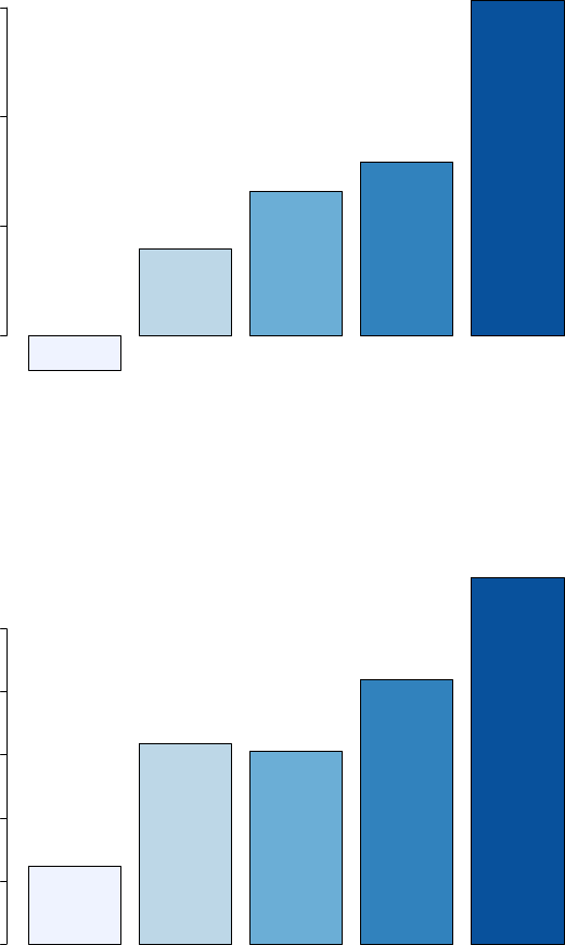
Figure A4: Sample Split by County-Level Minority Population Share
below .4% .4% to 1.2% 1.2% to 3.8% 3.8% to 14.3% above 14.3%
Assessment Gap for by Minority Population−Share Quintile
Quintile of County−Level Black Population Share
Assessment Ratio Difference
0.00 0.05 0.10 0.15
below 2.7% 2.7% to 6% 6% to 14.2% 14.2% to 32.1% above 32.1%
Assessment Gap for by Minority Population−Share Quintile
Quintile of County−Level Black or Hispanic Population Share
Assessment Ratio Difference
0.00 0.02 0.04 0.06 0.08 0.10
Note: These graphs show results from estimating the assessment gap in sub-samples by minority population
share at the county level. We split the sample into quintiles by on average county black or black and Hispanic
population share between 2005 to 2016. The quintile range is reflected below each bar. The regression output
underlying this table is shown in Table A4.
20

Table A1: Inequality for all other minority homeowners
log(Assessment Ratio)
(1) (2) (3)
Other Nonwhite Mortgage Holder 0.0278
∗∗∗
0.0198
∗∗∗
0.0190
∗∗∗
(0.0016) (0.0006) (0.0007)
Fixed Effects Jurisd-Yr Tract-Yr BG-Yr
No. Clusters 37723 37723 37723
Observations 6,987,915 6,987,915 6,987,915
R
2
0.8798 0.9005 0.9166
Note:
∗
p<0.1;
∗∗
p<0.05;
∗∗∗
p<0.01
Note: This table complements Table 2 and shows our baseline findings of a racial assessment gap for all other
minority homeowners. We regress the log assessment ratio on a set of fixed effects at the year × geography level
and on categorical groupings by racial and ethnic identity. Columns (1), (2), and (3) show results using fixed
effects at the jurisdiction-year, jurisdiction-tract-year, and jurisdiction-block group-year level, respectively. In all
columns, the reference group is non-Hispanic white residents. Standard errors are clustered at the jurisdiction
level.
21

Table A2: Assessment Ratio Differentials in California
log(Assessment) - log(Market)
(1) (2) (3)
Black Mortgage Holder 0.0413
∗∗∗
(0.0101)
Black or Hispanic Mortgage Holder 0.1060
∗∗∗
(0.0044)
Other Nonwhite Mortgage Holder 0.0653
∗∗∗
(0.0030)
Fixed Effects Jurisd-Year Jurisd-Year Jurisd-Year
No. Clusters 5603 5603 5603
Observations 1,186,388 1,186,388 1,186,388
R
2
0.3816 0.3820 0.3820
Note:
∗
p<0.1;
∗∗
p<0.05;
∗∗∗
p<0.01
Note: This table shows the results of our baseline assessment gap analysis for California alone. We regress the log
assessment ratio on a jurisdiction-year fixed effect and on categorical groupings by racial and ethnic identity. In
all columns, the reference group is non-Hispanic white residents, and for clarity coefficients for groups not being
considered in a given column are not reported. The estimates in this table reflect an assessment ratio differential
for the given grouping of minority residents relative to non-Hispanic white residents. Standard errors are clustered
at the jurisdiction level.
22

Table A3: Assessment Gap, Using Counties instead of Taxing Jurisdictions
log(Assessment Ratio)
(1) (2) (3)
Black Mortgage Holder 0.1687
∗∗∗
(0.0187)
Black or Hispanic Mortgage Holder 0.1356
∗∗∗
(0.0138)
Other Nonwhite Mortgage Holder 0.0321
∗∗∗
(0.0024)
Fixed Effects County-Year County-Year County-Year
No. Clusters 1982 1982 1982
Observations 6,987,915 6,987,915 6,987,915
R
2
0.8507 0.8508 0.8508
Note:
∗
p<0.1;
∗∗
p<0.05;
∗∗∗
p<0.01
Note: This table repeats our baseline assessment gap analysis, but uses county-year fixed effects rather than
jurisdiction-year. We regress the log assessment ratio on a county-year fixed effect and on categorical groupings
by racial and ethnic identity. In all columns, the reference group is non-Hispanic white residents, and for clarity
coefficients for groups not being considered in a given column are not reported. The estimates in this table
reflect an assessment ratio differential for the given grouping of minority residents, relative to non-Hispanic white
residents. Standard errors are clustered at the county level. This specification shows that our results are not
driven by the way we form jurisdictions. Our preferred specifications all use the more rigorous within-jurisdiction
analysis.
23

Table A4: Sample Split by County-Level Minority Population Share
Panel A
Assessment Value / Market Value
Quintile of County-Level Minority Population Share
(1) (2) (3) (4) (5)
Black Mortgage Holder −0.016 0.040
∗∗∗
0.066
∗∗∗
0.080
∗∗∗
0.153
∗∗∗
(0.054) (0.007) (0.004) (0.006) (0.021)
Fixed Effects Jurisd-Yr Jurisd-Yr Jurisd-Yr Jurisd-Yr Jurisd-Yr
No. Clusters 2087 6718 9619 12876 6445
Observations 54,188 412,164 919,591 3,129,016 2,472,956
R
2
0.857 0.938 0.905 0.888 0.847
Note:
∗
p<0.1;
∗∗
p<0.05;
∗∗∗
p<0.01
Panel B
Assessment Value / Market Value
Quintile of County-Level Minority Population Share
(1) (2) (3) (4) (5)
Black or Hispanic Mortgage Holder 0.025
∗
0.064
∗∗∗
0.061
∗∗∗
0.084
∗∗∗
0.116
∗∗∗
(0.013) (0.006) (0.003) (0.006) (0.018)
Fixed Effects Jurisd-Yr Jurisd-Yr Jurisd-Yr Jurisd-Yr Jurisd-Yr
No. Clusters 3452 6097 11116 12122 4969
Observations 78,526 303,353 1,443,303 2,803,100 2,359,633
R
2
0.816 0.784 0.860 0.879 0.881
Note:
∗
p<0.1;
∗∗
p<0.05;
∗∗∗
p<0.01
Note: Each panel shows the results from estimating the assessment gap on sub-samples based on county-level
demographics. For Panel A, we split our baseline sample into quintiles by average county black population share.
In Panel B the sample is split by black or Hispanic population share. In each panel, column 1 shows the estimated
assessment gap within the lowest minority-population quintile, and column 5 shows results for the highest quintile.
Regressions are run separately rather than pooled. We include jurisdiction-year fixed effects in all specifications.
Standard errors are clustered at the jurisdiction level.
24

Table A5: Hedonic Prices
Market Assessment Market Assessment
(1) (2) (3) (4)
Black Share −0.092
∗∗∗
−0.056
∗∗∗
(0.004) (0.004)
Black or Hispanic Share −0.117
∗∗∗
−0.078
∗∗∗
(0.006) (0.005)
Median HH Income 0.157
∗∗∗
0.144
∗∗∗
0.145
∗∗∗
0.135
∗∗∗
(0.008) (0.008) (0.008) (0.008)
Unemployment −0.027
∗∗∗
−0.013
∗∗∗
−0.030
∗∗∗
−0.015
∗∗∗
(0.003) (0.002) (0.004) (0.002)
SNAP Share −0.089
∗∗∗
−0.061
∗∗∗
−0.075
∗∗∗
−0.050
∗∗∗
(0.006) (0.004) (0.006) (0.004)
Owner Share −0.049
∗∗∗
−0.032
∗∗∗
−0.053
∗∗∗
−0.035
∗∗∗
(0.005) (0.003) (0.005) (0.004)
GINI 0.066
∗∗∗
0.059
∗∗∗
0.058
∗∗∗
0.053
∗∗∗
(0.004) (0.004) (0.004) (0.004)
Square Feet 0.256
∗∗∗
0.264
∗∗∗
0.256
∗∗∗
0.264
∗∗∗
(0.029) (0.030) (0.029) (0.030)
Bathrooms 0.107
∗∗∗
0.103
∗∗∗
0.107
∗∗∗
0.103
∗∗∗
(0.017) (0.017) (0.017) (0.017)
Year Built 0.031
∗∗∗
0.028
∗∗∗
0.030
∗∗∗
0.028
∗∗∗
(0.003) (0.003) (0.003) (0.003)
Other Attributes Y Y Y Y
Fixed Effects Jurisd-Year Jurisd-Year Jurisd-Year Jurisd-Year
No. Clusters 26152 26152 26152 26152
Observations 4,877,658 4,877,658 4,877,658 4,877,658
R
2
0.773 0.942 0.773 0.942
Note:
∗
p<0.1;
∗∗
p<0.05;
∗∗∗
p<0.01
Note: This table reports estimated hedonic prices from two separate hedonic models. The first model uses (log)
market as the dependent variable. These estimates are reported in columns 1 and 3. The second model uses
(log) assessed values as the dependent variable. These estimates are reported in columns 2 and 4. Otherwise,
the two hedonic models are identical: all regressors are the same. The table omits estimated coefficients for
indicator variables stating whether a property has a patio, pool, or fireplace. Standard errors are clustered at the
jurisdiction level. Figure 3 shows the difference between attribute-coefficients graphically.
25

Table A6: All Neighborhood Correlates
log(Assessment Ratio)
(1) (2)
Black Mortgage Holder 0.077
∗∗∗
(0.003)
Black Share 0.027
∗∗∗
(0.005)
Black or Hispanic Mortgage Holder 0.065
∗∗∗
(0.003)
Black or Hispanic Share 0.035
∗∗∗
(0.006)
Median HH Income −0.021
∗∗∗
−0.015
∗∗∗
(0.005) (0.004)
Unemployment 0.015
∗∗∗
0.017
∗∗∗
(0.004) (0.004)
SNAP Assistance 0.033
∗∗∗
0.030
∗∗∗
(0.004) (0.003)
Owner Percentage 0.021
∗∗∗
0.020
∗∗∗
(0.004) (0.004)
GINI Coef −0.011
∗∗∗
−0.009
∗∗∗
(0.002) (0.002)
Median Age 0.003
∗
0.008
∗∗∗
(0.002) (0.003)
Fixed Effects Jurisd-Year Jurisd-Year
No. Clusters 37679 37679
Observations 6,944,439 6,944,439
R
2
0.881 0.881
Note:
∗
p<0.1;
∗∗
p<0.05;
∗∗∗
p<0.01
Note: This table augments our baseline assessment gap findings in Table 2 with several measures of spatial
characteristics. All regressors are tract-level variables from the American Community Survey 5-year estimates.
Standard errors are clustered at the jurisdiction level. We continue to hold homeowner race fixed in this regression:
those coefficients are reported in the first line of notes immediately under the estimated coefficients. Standard
errors are clustered at the jurisdiction level.
26

Table A7: Assessment Gap by Segregation Decile
Panel A: Black Homeowners
log(Assessment Ratio)
(1) (2) (3) (4) (5) (6) (7) (8) (9) (10)
Black Mortgage Holder 0.0585
∗∗∗
0.0650
∗∗∗
0.0492
∗∗∗
0.0668
∗∗∗
0.0709
∗∗∗
0.0757
∗∗∗
0.0950
∗∗∗
0.0973
∗∗∗
0.1248
∗∗∗
0.1904
∗∗∗
(0.0140) (0.0063) (0.0083) (0.0051) (0.0076) (0.0069) (0.0176) (0.0101) (0.0103) (0.0371)
Fixed Effects Jur-Yr Jur-Yr Jur-Yr Jur-Yr Jur-Yr Jur-Yr Jur-Yr Jur-Yr Jur-Yr Jur-Yr
No. Clusters 418 1265 2036 3517 3454 4348 4341 6096 5875 6348
Observations 28,109 124,642 254,298 466,978 632,892 911,707 698,160 946,883 1,252,737 1,670,456
R
2
0.9246 0.8592 0.9008 0.9093 0.8849 0.9443 0.8785 0.8268 0.8603 0.8233
Note:
∗
p<0.1;
∗∗
p<0.05;
∗∗∗
p<0.01
Panel B: Black or Hispanic Homeowners
log(Assessment Ratio)
(1) (2) (3) (4) (5) (6) (7) (8) (9) (10)
Black or Hispanic Mortgage Holder 0.0718
∗∗∗
0.0464
∗∗∗
0.0518
∗∗∗
0.0503
∗∗∗
0.0461
∗∗∗
0.0565
∗∗∗
0.0531
∗∗∗
0.0586
∗∗∗
0.0838
∗∗∗
0.1509
∗∗∗
(0.0242) (0.0057) (0.0038) (0.0033) (0.0047) (0.0043) (0.0033) (0.0054) (0.0062) (0.0242)
Fixed Effects Jur-Yr Jur-Yr Jur-Yr Jur-Yr Jur-Yr Jur-Yr Jur-Yr Jur-Yr Jur-Yr Jur-Yr
No. Clusters 359 1393 2489 2513 3556 3125 3805 5329 6318 8811
Observations 11,241 66,821 210,686 239,072 376,861 329,217 595,845 1,166,829 1,672,469 2,317,821
R
2
0.9146 0.8489 0.9311 0.8870 0.8859 0.8956 0.9226 0.8598 0.9054 0.8332
Note:
∗
p<0.1;
∗∗
p<0.05;
∗∗∗
p<0.01
Note: This table provides point estimates for Figure 4 on the paper.
27

Table A8: Sample Split by Racial Attitudes
log(Assessment Ratio)
Baseline By Media Market By State
(1) (2) (3) (4) (5)
Black Mortgage Holder 0.128
∗∗∗
(0.015)
Black, High Animus 0.150
∗∗∗
0.070
∗∗∗
0.145
∗∗∗
0.076
∗∗∗
(0.022) (0.003) (0.011) (0.003)
Black, Low Animus 0.084
∗∗∗
0.055
∗∗∗
0.106
∗∗∗
0.049
∗∗∗
(0.008) (0.002) (0.033) (0.002)
Wald Test F-Stat N/A 8.13 14.55 1.24 55.61
Fixed Effects Jurisd-Yr Jursid-Yr Jurisd-Tract-Yr Jurisd-Yr Jursid-Tract-Yr
No. Clusters 37106 37106 37106 37106 37106
Observations 6,856,585 6,856,585 6,856,585 6,856,585 6,856,585
Note:
∗
p<0.1;
∗∗
p<0.05;
∗∗∗
p<0.01
Note: This table shows results of using the measures of racial animus described in Stephens-Davidowitz (2014)
to split our sample into regions of above- and below-median prejudice. Column 1 shows baseline results before
splitting the sample. Columns 2 and 3 use a media-market measure of animus. We use a Nielsen crosswalk to
associate media markets with individual counties. Columns 4 and 5 use a state-level measure of animus. For
each measure, the first result (column 2 or 4) shows the overall assessment gap. The second result shows the
homeowner effect estimated within jurisdiction-tract-year. For all specifications, standard errors are clustered at
the jurisdiction level.
28

Table A9: Robustness for Test of Transaction Prices
Assessment Gap Black Share B/H Share
(1) (2) (3) (4) (5) (6)
Black Seller 0.144
∗∗∗
0.117
∗∗∗
(0.015) (0.015)
Black or Hispanic Seller 0.110
∗∗∗
0.089
∗∗∗
(0.011) (0.011)
Test Sample −0.011
∗∗∗
−0.011
∗∗∗
(0.002) (0.002)
Sample Test Not Test Test Not Test Full Full
Fixed Effects Jurisd-Yr Jurisd-Yr Jurisd-Yr Jurisd-Yr Jurisd-Yr Jurisd-Yr
No. Clusters 18854 37193 18854 37193 37723 37723
Observations 2,135,966 4,851,949 2,135,966 4,851,949 6,987,915 6,987,915
R
2
0.910 0.870 0.910 0.870 0.618 0.686
Note:
∗
p<0.1;
∗∗
p<0.05;
∗∗∗
p<0.01
Note: This figure splits our core dataset to compare the assessment gap within the sample of homes used for our
test of racial differences in transaction prices (columns 1 and 3), and within the set which does not enter this test
(columns 2 and 4). Columns 5 and 6 regress Black share and Black or Hispanic share respectively on an indicator
for whether the observation is used in the test of transaction prices. All specifications include jurisdiction-year
fixed effects and standard errors are clustered at the jurisdiction level.
29

Table A10: Assessment Gap by Homeowner Tenure (Continuous)
log(Assessment) - log(Market)
(1) (2)
Black Mortgage Holder 0.1533
∗∗∗
(0.0180)
Black or Hispanic Mortgage Holder 0.1173
∗∗∗
(0.0120)
Years Since Sale 0.0049
∗∗∗
0.0052
∗∗∗
(0.0003) (0.0003)
Fixed Effects Jurisd-Year Jurisd-Year
No. Clusters 32705 32705
Observations 4,216,379 4,216,379
R
2
0.8939 0.8939
Note:
∗
p<0.1;
∗∗
p<0.05;
∗∗∗
p<0.01
Note: This table estimates the assessment gap with a continuous control for homeowner tenure (years since
purchase). Standard errors are clustered at the jurisdiction level.
30

Table A11: Assessment Gap Homeowner Tenure Bin
Panel A: Black Homeowners
log(Assessment) - log(Market)
1-5 Years 6-10 Years 10+ Years
Black Mortgage Holder 0.1435
∗∗∗
0.1630
∗∗∗
0.1368
∗∗∗
(0.0189) (0.0188) (0.0162)
Fixed Effects Jurisd-Year Jurisd-Year Jurisd-Year
No. Clusters 28682 27330 14874
Observations 2,313,454 1,546,116 356,809
R
2
0.9038 0.8866 0.9012
Note:
∗
p<0.1;
∗∗
p<0.05;
∗∗∗
p<0.01
Panel B: Black or Hispanic Homeowners
log(Assessment) - log(Market)
1-5 Years 6-10 Years 10+ Years
Black or Hispanic Mortgage Holder 0.1087
∗∗∗
0.1237
∗∗∗
0.0933
∗∗∗
(0.0122) (0.0133) (0.0106)
Fixed Effects Jurisd-Year Jurisd-Year Jurisd-Year
No. Clusters 28682 27330 14874
Observations 2,313,454 1,546,116 356,809
R
2
0.9037 0.8866 0.9011
Note:
∗
p<0.1;
∗∗
p<0.05;
∗∗∗
p<0.01
Note: This figure estimates the assessment gap by three homeowner tenure bins: 1-5 years, 6-10 years and greater
than 10 years. Regressions are run separately, rather than pooled. Standard errors are clustered at the jurisdiction
level.
31

Table A12: Effect of Black or Hispanic Ownership on Assessments
Assessments
Growth Levels
(1) (2) (3) (4)
Black Mortgage Holder 0.0711
∗
0.2917
∗∗∗
(0.0386) (0.0415)
Black or Hispanic Mortgage Holder 0.4103
∗∗∗
0.7923
∗∗∗
(0.0255) (0.0274)
Fixed Effects Two-Way Two-Way Two-Way Two-Way
No. Clusters 12268641 12268641 12268641 12268641
Observations 54,970,191 54,970,191 54,970,191 54,970,191
R
2
0.6925 0.6925 0.9910 0.9910
Note:
∗
p<0.1;
∗∗
p<0.05;
∗∗∗
p<0.01
Note: This table shows the results of a generalized difference-in-differences estimation. The dependent variable
is logged assessment value. Every home in this sample is transacted at least once. Fixed effects are two-way:
property and tract-year. In columns 1 and 2, the dependent variable is growth rates (log difference in assessed
value). In columns 3 and 4, the dependent variable is the logged assessment. Standard errors are clustered at the
property level.
32

Table A13: Assessment Ratio Pass Through to Tax Bill
Effective Tax Rate - Year of Sale (%)
Before Exemptions Before Exemptions Tax Bill
(1) (2) (3)
All Mortgage Holders 0.9842
∗∗∗
(0.0042)
White Mortgage Holder 0.9858
∗∗∗
0.9941
∗∗∗
(0.0038) (0.0041)
Black or Hispanic Mortgage Holder 0.9773
∗∗∗
0.9836
∗∗∗
(0.0067) (0.0069)
Other Nonwhite Mortgage Holder 0.9823
∗∗∗
0.9892
∗∗∗
(0.0042) (0.0043)
Fixed Effects Jurisd-Year Jurisd-Year Jurisd-Year
No. Clusters 34776 34776 34776
Observations 5,574,777 5,574,777 5,574,777
R
2
0.9096 0.9097 0.8658
Note:
∗
p<0.1;
∗∗
p<0.05;
∗∗∗
p<0.01
Note: This table shows the results of regressing log effective tax rate on log assessment ratio. Column 1 presents
estimates for all homeowners. Columns 2 and 3 show a breakdown by racial and ethnic grouping. Results for
black homeowners alone are very similar to those reported here. In columns 1 and 2, the dependent variable
is an effective rate formed using the gross (pre-exemption) tax bill reported in the ATTOM dataset. Column
3 computes a post-exemption effective rate by subtracting reported exemptions from the reported tax bill. The
effective rate is computed by using the tax bill reported in the same year as the sale. All specifications use
jurisdiction-year fixed effects. Standard errors are clustered at the jurisdiction level.
33

Table A14: Effective Tax Rate, Sale Year
Effective Tax Rate - In Sale Year (%)
Assmt. Gap Before Exemptions Tax Bill Assmt. Gap Before Exemptions Tax Bill
(1) (2) (3) (4) (5) (6)
Black Mortgage Holder 13.6796
∗∗∗
15.3594
∗∗∗
15.8591
∗∗∗
(2.0953) (2.1055) (2.1254)
Black or Hispanic Mortgage Holder 10.1349
∗∗∗
11.2948
∗∗∗
11.6403
∗∗∗
(1.5904) (1.5689) (1.5320)
Jurisd-Year FE Y Y Y Y Y Y
No. Clusters 25267 25267 25267 25267 25267 25267
Observations 3,027,748 3,027,748 3,027,748 3,027,748 3,027,748 3,027,748
R
2
0.8956 0.6961 0.6488 0.8955 0.6958 0.6484
Note:
∗
p<0.1;
∗∗
p<0.05;
∗∗∗
p<0.01
Note: This table repeats our baseline estimation, but uses effective tax rate as the dependent variable instead
of assessment ratio. Coefficients are percentages. For each racial and ethnic grouping, we present two sets of
results. In odd columns, we show results using an effective rate computed using the gross (pre-exemption) tax
bill and observed market value in the same year. In even columns, we compute a post-exemption effective tax
rate, by subtracting reported exemptions from the gross tax bill, and then dividing by market value. We trim any
observation above a calculated effective tax rate of 25% both before and net of exemptions. We believe this to be
a conservative choice as 25% is far higher than any property tax rate of which we are aware (the national median
is approximately 1.4%), and is more likely than not to be a data error. All specifications use jurisdiction-year
fixed effects to hold constant the level of intended taxation. Standard errors are clustered at the jurisdiction level.
34

Table A15: Effective Tax Rate, One Year Before Sale
Effective Tax Rate - One Year Before Sale (%)
Before Exemptions Tax Bill Before Exemptions Tax Bill
(1) (2) (3) (4)
Black Mortgage Holder 15.8285
∗∗∗
16.5085
∗∗∗
(2.2103) (2.2371)
Black or Hispanic Mortgage Holder 11.6723
∗∗∗
12.2055
∗∗∗
(1.6216) (1.6311)
Jurisd-Year FE Y Y Y Y
No. Clusters 25267 25267 25267 25267
Observations 3,027,748 3,027,748 3,027,748 3,027,748
R
2
0.6798 0.6324 0.6795 0.6321
Note:
∗
p<0.1;
∗∗
p<0.05;
∗∗∗
p<0.01
Note: This table repeats our analysis in Table A14, but uses the tax bill from the year before sale. The denominator
for computing the effective tax rate remains the observed market value. Coefficients are percentages. For each
racial and ethnic grouping we present two sets of results.In odd columns, we show results using an effective rate
computed using the gross (pre-exemption) tax bill and observed market value in the same year. In even columns,
we compute a post-exemption effective tax rate, by subtracting reported exemptions from the gross tax bill, and
then dividing by market value. We trim any observation above a calculated effective tax rate of 25% both before
and net of exemptions. We believe this to be a conservative choice as 25% is far higher than any property tax
rate of which we are aware (the national median is approximately 1.4%), and is more likely than not to be a
data error. All specifications use jurisdiction-year fixed effects to hold constant the level of intended taxation.
Standard errors are clustered at the jurisdiction level.
35

Table A16: Effective Tax Rate, One Year After Sale
Effective Tax Rate - One Year After Sale (%)
Before Exemptions Tax Bill Before Exemptions Tax Bill
(1) (2) (3) (4)
Black Mortgage Holder 13.6175
∗∗∗
13.9837
∗∗∗
(1.9898) (1.9776)
Black or Hispanic Mortgage Holder 9.9325
∗∗∗
10.1185
∗∗∗
(1.4818) (1.4179)
Jurisd-Year FE Y Y Y Y
No. Clusters 25267 25267 25267 25267
Observations 3,027,748 3,027,748 3,027,748 3,027,748
R
2
0.7155 0.6599 0.7152 0.6595
Note:
∗
p<0.1;
∗∗
p<0.05;
∗∗∗
p<0.01
Note: This table repeats our analysis in Table A14, but uses the tax bill from the year after the sale. The
denominator for computing the effective tax rate remains the observed market value. Coefficients are percentages.
For each racial and ethnic grouping we present two sets of results. In odd columns, we show results using an
effective rate computed using the gross (pre-exemption) tax bill and observed market value in the same year. In
even columns, we compute a post-exemption effective tax rate, by subtracting reported exemptions from the gross
tax bill, and then dividing by market value. We trim any observation above a calculated effective tax rate of 25%
both before and net of exemptions. We believe this to be a conservative choice as 25% is far higher than any
property tax rate of which we are aware (the national median is approximately 1.4%), and is more likely than
not to be a data error. All specifications use jurisdiction-year fixed effects to hold constant the level of intended
taxation. Standard errors are clustered at the jurisdiction level.
36

Table A17: Synthetic Assessments Using Zip Code HPIs
log(Assessment) - log(Market)
Real Assessments Synthetic Assessments
(1) (2) (3) (4)
Black Mortgage Holder 0.144
∗∗∗
−0.041
∗∗∗
(0.015) (0.003)
Black or Hispanic Mortgage Holder 0.110
∗∗∗
−0.051
∗∗∗
(0.011) (0.003)
Jurisd-Year FE Y Y Y Y
No. Clusters 18853 18853 18853 18853
Observations 2,135,943 2,135,943 2,135,943 2,135,943
R
2
0.910 0.910 0.712 0.713
Note:
∗
p<0.1;
∗∗
p<0.05;
∗∗∗
p<0.01
Note: This table shows the results from our proposed approach for correcting the assessment gap. Using the
algorithm described in Section C.v, we construct synthetic assessments using zip-code-level HPIs. We use Zillow’s
publicly available ZHVI series by zip-code. Our approach uses an initial transaction to pin down the base assess-
ment value. At every subsequent transaction, we observe a realized assessment ratio along with our synthetically
constructed assessment ratio. Columns 1 & 2 show that the overall assessment gap looks similar in the subset
of homes to which can we apply this approach (smaller chiefly because the first transaction is not included in
the analysis). Columns 3 & 4 show the assessment gap using our synthetic assessment ratios. All specifications
include jurisdiction-year fixed effects. Standard errors are clustered at the jurisdiction level.
37

Table A18: Synthetic Assessments, Stopping Growth in January Each Year
log(Assessment) - log(Market)
Real Assessments Synthetic Assessments
(1) (2) (3) (4)
Black Mortgage Holder 0.144
∗∗∗
−0.040
∗∗∗
(0.015) (0.003)
Black or Hispanic Mortgage Holder 0.110
∗∗∗
−0.049
∗∗∗
(0.011) (0.003)
Jurisd-Year FE Y Y Y Y
No. Clusters 18853 18853 18853 18853
Observations 2,135,943 2,135,943 2,135,943 2,135,943
R
2
0.910 0.910 0.692 0.693
Note:
∗
p<0.1;
∗∗
p<0.05;
∗∗∗
p<0.01
Note: This table shows an alternative implementation of our proposed approach for correcting the assessment
gap. The analysis in Table A17 uses constructed assessments which increase with the zip-code HPI until the
month of sale. In this table, we use constructed assessments which change only in January of each year. This
more closely parallels the actual assessment practice of generating a single value each year. In this approach, when
a sale occurs, the assessment is out of date by up to 12 months. Columns 1 & 2 are identical to Table A17 and
show that the overall assessment gap looks similar in the subset of homes to which we can apply this approach.
Columns 3 & 4 show the assessment gap using January-revised synthetic assessments. All specifications include
jurisdiction-year fixed effects. Standard errors are clustered at the jurisdiction level.
38

Table A19: Effect of Assessment Caps on Inequality
log(Assessment Ratio)
No Cap Cap Exists Cap Exists and Binds
(1) (2) (3)
Panel A: Black Homeowners
Black Mortgage Holder 0.1591
∗∗∗
0.0979
∗∗∗
0.0798
∗∗∗
(0.0232) (0.0060) (0.0067)
Panel B: Black or Hispanic Homeowners
Black or Hispanic Mortgage Holder 0.1225
∗∗∗
0.0844
∗∗∗
0.0574
∗∗∗
(0.0177) (0.0044) (0.0041)
Fixed Effects Jurisd-Year Jurisd-Year Jurisd-Year
No. Clusters 29020 8934 4423
Observations 4,172,149 2,149,582 506,051
Note:
∗
p<0.1;
∗∗
p<0.05;
∗∗∗
p<0.01
Note: This table shows our findings of a racial assessment gap in areas with different policies regarding a cap
rate of growth. Panel A presents our results for Black homeowners, and Panel B presents our results for Black or
Hispanic homeowners. In all specifications, we regress the log assessment ratio on jurisdiction-year fixed effects
and on categorical groupings by racial and ethnic identity. Column (1), (2), and (3) respectively present results
for areas with no known cap policy, areas with a cap, and areas with a cap that is binding. In all columns,
the reference group is non-Hispanic white residents, and for clarity coefficients for groups not being considered
in a given column are not reported. The estimates in this table reflect an assessment ratio differential for the
given grouping of minority residents relative to non-Hispanic white residents. Standard errors are clustered at the
jurisdiction level.
39

Table A20: Assessment Gap by Reassessment Cycle
log(Assessment Ratio)
1yr 2yrs 3yrs 4yrs 5yrs 6yrs 8yrs 9yrs none
(1) (2) (3) (4) (5) (6) (7) (8) (9)
Panel A: Black Homeowners
Black Mortgage Holder 0.1081
∗∗∗
0.1113
∗∗∗
0.1855
∗∗
0.1277
∗∗∗
0.1565
∗∗∗
0.1919
∗∗∗
0.1202
∗∗∗
0.1231
∗∗∗
0.2502
∗∗∗
(0.0078) (0.0337) (0.0833) (0.0186) (0.0250) (0.0323) (0.0156) (0.0224) (0.0447)
Panel B: Black or Hispanic Homeowners
Black or Hispanic Mortgage Holder 0.0898
∗∗∗
0.0892
∗∗∗
0.1420
∗∗∗
0.1017
∗∗∗
0.1055
∗∗∗
0.1504
∗∗∗
0.1026
∗∗∗
0.1096
∗∗∗
0.1970
∗∗∗
(0.0056) (0.0189) (0.0530) (0.0117) (0.0206) (0.0300) (0.0142) (0.0226) (0.0449)
Fixed Effects Jurisd-Year Jurisd-Year Jurisd-Year Jurisd-Year Jurisd-Year Jurisd-Year Jurisd-Year Jurisd-Year Jurisd-Year
No. Clusters 11686 3867 4424 7887 5639 5636 1783 66 2358
Observations 2,437,030 701,784 880,924 558,264 863,890 545,436 231,146 35,077 68,180
Note:
∗
p<0.1;
∗∗
p<0.05;
∗∗∗
p<0.01
Note: This table shows our findings of a racial assessment gap in areas with different reassessment cycles. Panel A
presents our results for Black homeowners, and Panel B presents our results for Black or Hispanic homeowners. In
all specifications, we regress the log assessment ratio on jurisdiction-year fixed effects and on categorical groupings
by racial and ethnic identity. Columns (1)–(8) present results for areas with a reassessment cycle in place but with
varying cycle lengths. Column (9) presents results for areas with no reassessment cycles in place. In all columns,
the reference group is non-Hispanic White residents, and for clarity coefficients for groups not being considered
in a given column are not reported. The estimates in this table reflect an assessment ratio differential for the
given grouping of minority residents relative to non-Hispanic White residents. Standard errors are clustered at
the jurisdiction level.
40
