Frank E. Harrell, Jr. With Applications to Linear Models, Logistic and

Regression

Modeling

Strategies

Frank E. Harrell, Jr.

With Applications to Linear Models,

Logistic and Ordinal Regression,

and Survival Analysis

Second Edition

Springer Series in Statistics

Advisors:

P. Bickel, P. Diggle, S.E. Feinberg, U. Gather,

I. Olkin, S. Zeger

More information about this series at

http://www.springer.com/series/692

Frank E. Harrell, Jr.

Regression Modeling

Strategies

With Applications to Linear Models,

Logistic and Ordinal Regression,

and Survival Analysis

Second Edition

123

Frank E. Harrell, Jr.

Department of Biostatistics

School of Medicine

Vanderbilt University

Nashville, TN, USA

ISSN 0172-7397 ISSN 2197-568X (electronic)

Springer Series in Statistics

ISBN 978-3-319-19424-0 ISBN 978-3-319-19425-7 (eBook)

DOI 10.1007/978-3-319-19425-7

Library of Congress Control Number: 2015942921

Springer Cham Heidelberg New York Dordrecht London

This work is subject to copyright. All rights are reserved by the Publisher, whether the whole or part of

the material is concerned, speciﬁcally the rights of translation, reprinting, reuse of illustrations, recitation,

broadcasting, reproduction on microﬁlms or in any other physical way, and transmission or information

storage and retrieval, electronic adaptation, computer software, or by similar or dissimilar methodology

now known or hereafter developed.

The use of general descriptive names, registered names, trademarks, service marks, etc. in this publication

does not imply, even in the absence of a speciﬁc statement, that such names are exempt from the relevant

protective laws and regulations and therefore free for general use.

The publisher, the authors and the editors are safe to assume that the advice and information in this book

are believed to be true and accurate at the date of publication. Neither the publisher nor the authors or

the editors give a warranty, express or implied, with respect to the material contained herein or for any

errors or omissions that may have been made.

Printed on acid-free paper

Springer International Publishing AG Switzerland is part of Springer Science+Business Media (

www.

springer.com

)

To the memories of Frank E. Harrell, Sr.,

Richard Jackson, L. Richard Smith, John

Burdeshaw, and Todd Nick, and with

appreciation to Liana and Charlotte

Harrell, two high school math teachers:

Carolyn Wailes (n´ee Gaston) and Floyd

Christian, two college professors: David

Hurst (who advised me to choose the ﬁeld

of biostatistics) and Doug Stocks, and my

graduate advisor P. K. Sen.

Preface

There are many books that are excellent sources of knowledge abo ut

individual statistical tools (survival models, general linear models, etc.), but

the art of data analysis is about choosing and using multiple tools. In the

words of Chatﬁeld [

100, p. 420] “...students typically know the technical de-

tails of regression for example, but not necessarily when and how to apply it.

This argues the need for a better balance in the literature a nd in statistical

teaching between techniques and problem solving strategies.” Whether ana-

lyzing risk factors, adjusting for biases in observational studies, or developing

predictive models, there are common problems that few regression texts ad-

dress. For example, there are missing data in the majority of datasets one is

likely to encounter (other than those used in textbooks!) but most r e gression

texts do not include methods for dealing with such data eﬀectively, and most

texts on missing data do not cover regression modeling.

This book links standard regression modeling approaches with

• methods for relaxing linearity assumptio ns that still allow one to easily

obtain predictions and conﬁdence limits for future observations, and to do

formal hypothesis tests,

• non-additive modeling approaches not requiring the assumption that

interactions are always linear × linear,

• methods for imputing missing data and for penalizing variances for incom-

plete data,

• methods for handling large numbers of predictors without resorting to

problematic stepwise variable selection techniques,

• data reduction methods (unsupervised learning methods, some of which

are based on multivariate psychometric techniques too seldom used in

statistics) that help with the problem of“too many variables to analyze and

not enough o bservations” as well as making the model more interpretable

when there are predictor variables containing overlapping information,

• methods for quantifying predictive accuracy of a ﬁtted model,

vii

viii Preface

• powerful model validation techniques based on the bootstrap that allow the

analyst to estimate predictive accuracy nearly unbiasedly without holding

back data from the model development process, and

• graphical methods for understanding complex models.

On the last p o int, this text has special emphasis on what could b e called

“presentation graphics for ﬁtted mo dels” to help make regression analyses

more palatable to non-statisticians. For example, nomograms have long been

used to make equations portable, but they are not drawn r outinely because

doing so is very labor-intensive. An

R function called nomogram in the package

described below draws nomograms from a regression ﬁt, and these diagrams

can be used to communicate modeling results as well as to obtain predicted

values manually even in the presence of complex variable transformations.

Most of the methods in this text apply to all regression models, but special

emphasis is given to some of the most popular ones: multiple regression using

least squares and its generalized least squares extension for serial (rep eated

measurement) da ta, the binary logistic model, models for ordinal responses,

parametric surviva l regression models, and the Cox semiparametric survival

model. There is also a chapter on nonparametric transform-both-sides regres-

sion. Emphasis is given to detailed case studies for these methods as well as

for data reduction, imputation, model simpliﬁcation, an d other tasks. Ex-

cept for the case study on survival of Titanic passengers, all examples are

from biomedical research. However, the methods presented here have broad

application to other areas including economics, epidemiology, sociology, psy-

chology, engineering, and predicting consumer behavior and other business

outcomes.

This text is intended for Masters o r PhD level graduate students who

have had a general introductor y probability and statistics course and who

are well versed in ordinary multiple regression and intermediate algebra. The

book is also intended to serve as a reference for data analysts and statistical

methodologists. Readers without a strong background in applied statistics

may wish to ﬁrst study one of the many introductory applied statistics and

regression texts that are available. The author’s course notes Biostatistics

for Biomedical Research on the text’s web site covers basic regression and

many other topics. The paper by Nick and Hardin

[

476] also provides a good

introduction to multivariable modeling and interpretation. There are many

excellent intermediate level texts on regressio n analysis. One of them is by

Fox, which also has a companion software-based text [

200, 201]. For readers

interested in medical or epidemiologic research, Steyerberg’s excellent text

Clinical Pre diction Models [

586] is an ide al companion for Regression Modeling

Strategies. Steyerberg’s book provides further explanations, examples, and

simulations of many of the methods presented here. And no text on regression

modeling should fail to mention the seminal work of John Nelder [

450].

The overall philosophy of this book is summarized by the following state-

ments.

Preface ix

• Satisfaction of model assumptions improves precision and increases statis-

tical power.

• It is more productive to make a model ﬁt step by step (e.g., transformation

estimation) than to postulate a simple model and ﬁnd out what went

wrong.

• Graphical methods should be married to formal inference.

• Overﬁtting occurs frequently, so data reduction and mo del validation are

important.

• In most research projects, the cost of data collection far outweighs the cost

of data analysis, so it is important to use the most eﬃcient and accurate

modeling techniques, to avoid categorizing continuous variables, and to

not remove data from the estimation sample just to be able to validate the

model.

• The b ootstrap is a breakthrough for statistical modeling, and the analyst

should use it for many steps of the modeling strategy, including deriva-

tion of distribution-free conﬁdence intervals and estimation of optimism

in model ﬁt that takes into account variations caused by the modeling

strategy.

• Imputation of missing data is better than discarding incomplete observa-

tions.

• Variance often dominates bias, so biased methods such as penalized max-

imum likelihood estimation yield models that have a greater chance of

accurately predicting future observations.

• Software without multiple facilities for assessing and ﬁxing model ﬁt may

only seem to be user-friendly.

• Carefully ﬁtting an improper model is better than badly ﬁtting (and over-

ﬁtting) a well-chosen one.

• Methods that work for all types of regression models are the most valuable.

• Using the data to guide the data analysis is almost as dangerous as not

doing so.

• There are beneﬁts to modeling by deciding how many degrees of freedom

(i.e., number of regression parameters) can be “spent,”deciding where they

should be sp ent, and then spending them.

On the last point, the author believes that signiﬁcance tests and P -values

are problematic, especia lly when making modeling decisions. Judging by the

increased emphasis o n conﬁdence intervals in scientiﬁc journals there is reason

to believe that hypothesis testing is gradually being de-emphasized. Yet the

reader will notice that this text contains many P -values. How do e s that make

sense when, for example, the text recommends against simplifying a mo del

when a test of linear ity is not signiﬁcant? First, some rea ders may wish to

emphasize hypothesis testing in general, and some hypotheses have special

interest, such as in pharmaco logy where one may be interested in whether

the eﬀect of a drug is linear in log dose. Second, many of the more interesting

hypothesis tests in the text are tests of complexity (nonlinearity, interaction)

of the overall model. Null hypotheses of linearity of eﬀects in particular are

x Preface

frequently rejected, providing formal evidence that the analyst’s investment

of time to use more than simple statistical models was warranted.

The rapid development of Bayesian modeling methods and rise in their use

is exciting. Full Bayesian modeling greatly reduces the need for the approxi-

mations made for conﬁdence intervals and distributions of test statistics, a n d

Bayesian metho ds formalize the still rather ad hoc frequentist approach to

penalized maximum likelihood estimation by using skeptical prior distribu-

tions to obtain well-deﬁned posterior distributio ns that automatically deal

with shrinkage. The Bayesian approach also provides a formal mechanism for

incorporating information external to the data. Although Bayesian methods

are beyond the scope of this text, the text is Bayesian in spirit by emphasizing

the careful use of subject matter expertise while building statistical models.

The text emphasizes predictive modeling, but as discussed in Chapter

developing go od predictions goes hand in hand with accurate estimation of

eﬀects and with hypothesis testing (when appropriate). Besides emphasis

on multivariable modeling, the text includes a Chapter

17 introducing sur-

vival analysis and methods for analyzing various types of single and multiple

events.Thisbookdoesnotprovideexamplesofanalysesofonecommon

type of response variable, namely, cost and related measures of resource con-

sumption. However, least squares modeling presented in Chapter

15.1,the

robust r ank-based methods presented in Chapters

13, 15,and20,andthe

transform-both-sides regression models discussed in Chapter 16 are very ap-

plicable and robust for modeling economic o utcomes. See

[

167] and [260] for

example analyses of such dependent variables using, respectively, the Cox

model and nonparametric additive regression. The central Web site for this

book (see the App endix) has much more material on the use of the Cox model

for analyzing costs.

This text does not address some important study design issues that if not

respected can doom a predictive modeling or estimation project to failure.

See Laupacis, Sekar , and Stiell

[

378] for a list of some of these issues.

Heavy use is made of the S language used by R. R is the focus because

it is an elegant object-oriented system in which it is easy to implement new

statistical ideas. Many R users a round the world have done so, and their work

has beneﬁted many of the procedures described here. R also has a uniform

syntax for specifying statistical models (with respect to categorical predictors,

interactions, etc.), no matter which type of model is being ﬁtted [

96].

The free, open-source statistical software system R has been adopted by

analysts and resear ch statisticians worldwide. Its capabilities are growing

exponentially because of the involvement of an ever-growing community of

statisticians who are adding new tools to the base R system through con-

tributed packages. All of the functions used in this text are available in R.

See the boo k’s Web site for updated information about software availability.

Readers who don’t use R or any other statistical software environment will

still ﬁnd the statistical methods and case studies in this text useful, and it is

hoped that the code that is presented will make the statistical methods more

Preface xi

concrete. At the very least, the code demonstrates that all of the methods

presented in the text are feasible.

This text does not teach analysts how to use R. For that, the reader may

wish to see reading recommendations on www.r-project.org as well as Venables

and Ripley [

635] (which is also an excellent companion to this text) and the

many other excellent texts on R. See the Appendix for more information.

In addition to p owerful features that are built into R,thistextusesa

package of freely available R functions called rms written by the author. rms

tracks modeling details related to the expanded X or design matrix. It is a

series of over 200 functions for model ﬁtting, testing, estimation, validation,

graphics, prediction, and typesetting by storing enhanced model design at-

tributes in the ﬁt.

rms includes functions for least squares and penalized least

squares multiple regression modeling in addition to functions for binary and

ordinal r egression, generalized least squares for analyzing serial data, quan-

tile regression, and survival analysis that are emphasized in this text. Other

freely available miscellaneous R functions used in the text are found in the

Hmisc package also written by the author. Functions in Hmisc include facilities

for data reduction, imputation, power and sample size calculation, advanced

table making, recoding variables, impo rting and inspecting data, and general

graphics. Consult the Appendix for information o n obtaining

Hmisc and rms.

The author and his colleagues have written SAS macros for ﬁtting re-

stricted cubic splines and for other basic operations. See the Appendix for

more information. It is unfair not to mention some excellent capabilities of

other statistical packages such as Stata (which has also been extended to

provide regression splines and other modeling tools), but the extendability

and graphics of

R makes it especially attractive for all aspects of the compre-

hensive modeling strategy presented in this book.

Portions of Chapters

4 and 20 were published as reference [269].Someof

Chapter 13 was published as reference [272].

The author may be contacted by electronic mail at f.harrell@

vanderbilt.edu

and would appreciate being informed of unclear points, er-

rors, and omissions in this book. Suggestions for improvements and for future

topics are also welcome. As describ ed in the Web site, instructors may con-

tact the author to obtain copies of quizzes and extra assignments (both with

answers) related to much of the material in the earlier chapters, and to obtain

full solutions (with graphical output) to the majority of assignments in the

text.

Major changes since the ﬁrst edition include the following:

1. Creation of a now mature

R package, rms, that replaces and greatly ex-

tends the Design library used in the ﬁrst edition

2. Conversion of all of the book’s c ode to R

3. Conversion of the book source into knitr [

677] reproducible documents

4. All code from the text is executable and is on the web site

5. Use of color graphics and use of the ggplot2 graphics package [667]

6. Scanned images were re-drawn

xii Preface

7. New text about problems with dichotomization of continuous variables

and with classiﬁcation (as opp o sed to prediction)

8. Expanded material on multiple imputation and predictive mean match-

ing and emphasis on multiple imputation (using the Hmisc aregImpute

function) instead of single imputation

9. Addition of redundancy analysis

10. Added a new section in Chapter

5 on bootstr ap conﬁdence intervals for

rankings of predictors

11. Replacement of the U.S. presidential electio n data with a nalyses of a new

diabetes dataset from NHANES using ordina l and quantile regression

12. More emphasis o n semiparametric ordinal regression models for contin-

uous Y , as direct competitors of ordinary multiple regression, with a

detailed case study

13. A new chapter on generalized least squares for analysis of serial response

data

14. The case study in imputatio n and data reduction was completely reworked

and now focuses only on data reduction, with the addition of sparse prin-

cipal components

15. More information about indexes of predictive accuracy

16. Augmentation of the chapter on maximum likelihood to include more

ﬂexible ways of testing contrasts as well as new metho ds for obtaining

simultaneous conﬁdence intervals

17. Binary logistic regression case study 1 was completely re-worked, now

providing examples of model selection and mo del approxima tion accuracy

18. Single imputation was dropped from binary logistic case study 2

19. The case study in transform-both-sides regression modeling has been re-

worked using simulated data where true transformations are known, and

a new example of the smearing estimator was added

20. Addition of 225 references, most of them published 2001–2014

21. New guidance on minimum sample sizes needed by some of the models

22. De-emphasis of bootstrap bumping

[

610] for obtaining simultaneous con-

ﬁdence regions, in favor of a gener al multiplicity approach [307].

Acknowledgments

A good deal of the writing of the ﬁrst edition of this book was done during

my 17 years on the faculty of Duke University. I wish to thank my close col-

league Kerry Lee for providing many valuable ideas, fruitful collab o rations,

and well-organized lecture notes from which I have greatly b eneﬁted over the

past years. Terry Therneau of Mayo Clinic has given me many of his wonderful

ideas for many years, and has written state-of-the-art

R software for survival

analysis that forms the core of survival analysis software in my rms package.

Michael Symons of the Department of Biostatistics of the University of North

Preface xiii

Carolina at Chapel Hill and Timothy Morgan of the Division of Public Health

Sciences a t Wake Forest University School of Medicine also provided course

materials, some of which motivated portions of this text. My former clini-

cal colleagues in the Cardiology Division at Duke University, Rob ert Caliﬀ,

Phillip Harris, Mark Hlatky, Dan Mark, David Pryor, and Robert Rosati,

for many years provided valuable motivation, feedback, and ideas through

our interaction on clinical problems. Besides Kerry Lee, statistical colleagues

L. Richard Smith, Lawrence Muhlbaier, and Elizabeth DeLong clariﬁed my

thinking and gave me new ideas on numerous occasions. Charlotte Nelson

and Carlos Alzola frequently helped me debug S routines when they thought

they were just analyzing data.

Former students Bercedis Peterson, James Herndon, Robert McMahon,

and Yuan-Li Shen have provided many insights into logistic and survival mod-

eling. Associations with Doug Wagner and William Knaus of the University

of Virginia, Ken Oﬀord of Mayo Clinic, David Naftel of the University of Al-

abama i n Birmingham, Phil Miller of Washington University, and Phil Good-

man of the University of Nevada Reno have provided many valuable ideas and

motivations for this work, as have Michael Schemper of Vienna University,

Janez Sta re of Ljubljana University, Slovenia, Ewout Steyerb erg of Erasmus

University, Rotterdam, Karel Moons of Utrecht University, and Drew Levy of

Genentech. Richard Goldstein, along with several anonymous reviewers, pro-

vided many helpful criticisms o f a previous version of this manuscript that

resulted in signiﬁcant improvements, and critical reading by Bob Edson (VA

Co operative Studies Program, Palo Alto) resulted in many error corrections.

Thanks to Brian Ripley of the University of Oxford for providing ma ny help-

ful software tools and statistical insights that greatly aided in the production

of this book, and to Bill Venables of CSIRO Australia for wisdom, both sta-

tistical and otherwise. This work would also not have b een possible without

the S environment developed by Rick Becker, John Chambers, Allan Wilks,

and the

R language developed by Ross Ihaka and Robert Gentleman.

Work for the second edition was done in the excellent academic environ-

ment of Vanderbilt University, where biostatistical and biomedical co lleagues

and graduate students provided new insig hts and stimulating discussions.

Thanks to Nick Cox, Durham University, UK, who provided from his careful

reading of the ﬁrst edition a very large number of improvements and correc-

tions that were incorporated into the second. Four anonymous reviewers of

the second edition also made numerous suggestions that improved the text.

Nashville, TN, USA Frank E. Harrell, Jr.

July 2015

Contents

Typographical Conventions ................................... xxv

1 Introduction .............................................. 1

1.1 Hypothesis Testing, Estimation, and Prediction ........... 1

1.2 Examples of Uses of Predictive Multivariable Modeling ..... 3

1.3 Prediction vs. Classiﬁcation ............................. 4

1.4 Planning for Modeling ................................. 6

1.4.1 Emphasizing Continuous Variables ............... 8

1.5 Choice of the Model ................................... 8

1.6 Further Reading ....................................... 11

2 General Aspects of Fitting Regression Models ............ 13

2.1 Notation for Multivariable Regression Models ............. 13

2.2 Model Formulations ................................... 14

2.3 Interpreting Model Parameters .......................... 15

2.3.1 Nominal Predictors ............................. 16

2.3.2 Interactions.................................... 16

2.3.3 Example: Inference for a Simple Model ............ 17

2.4 Relaxing Linearity Assumption for Continuous Predictors .. 18

2.4.1 Avoiding Categorization ......................... 18

2.4.2 Simple Nonlinear Terms ......................... 21

2.4.3 Splines for Estimating Shape of Regression

Function and Determining Predictor

Transformations

................................ 22

2.4.4 Cubic Spline Functions .......................... 23

2.4.5 Restricted Cubic Splines ........................ 24

2.4.6 Choosing Number and Position of Knots .......... 26

2.4.7 Nonparametric Regression ....................... 28

2.4.8 Advantages of Regression Splines over

Other Methods ................................. 30

xvi Contents

2.5 Recursive Partitioning: Tree-Based Models ................ 30

2.6 Multiple Degree of Freedom Tests of Association .......... 31

2.7 Assessment of Model Fit ............................... 33

2.7.1 Regression Assumptions ......................... 33

2.7.2 Modeling and Testing Complex Interactions ....... 36

2.7.3 Fitting Ordinal Predictors ....................... 38

2.7.4 Distributional Assumptions ...................... 39

2.8 Further Reading ....................................... 40

2.9 P roblems ............................................. 42

3 Missing Data ............................................. 45

3.1 Types of Missing Data ................................. 45

3.2 Prelude to Modeling ................................... 46

3.3 Missing Values for Diﬀerent Types of Response Variables ... 47

3.4 Problems with Simple Alternatives to Imputation ......... 47

3.5 Strategies for Developing an Imputation Model ............ 49

3.6 Single Conditional Mean Imputation ..................... 52

3.7 Predictive Mean Matching .............................. 52

3.8 Multiple Imputation ................................... 53

3.8.1 The

aregImpute and Other Chained Equations

Approaches

.................................... 55

3.9 Diagnostics ........................................... 56

3.10 Summary and Rough Guidelines......................... 56

3.11 Further Reading ....................................... 58

3.12 Problems ............................................. 59

4 Multivariable Modeling Strategies ........................ 63

4.1 Prespeciﬁcation of Predictor Complexity Without

Later Simpliﬁcation

.................................... 64

4.2 Checking Assumptions of Multiple Predictors

Simultaneously

........................................ 67

4.3 Variable Selection ..................................... 67

4.4 Sample Size, Overﬁtting, and Limits on Number

of Predictors .......................................... 72

4.5 Shrinkage ............................................ 75

4.6 Collinearity ........................................... 78

4.7 Data Reduction ....................................... 79

4.7.1 Redundancy Analysis ........................... 80

4.7.2 Va riable Clustering ............................. 81

4.7.3 Transformation and Scaling Variables Without

Using Y

....................................... 81

4.7.4 Simultaneous Transformation and Imputation ...... 83

4.7.5 Simple Scoring of Variable Clusters ............... 85

4.7.6 Simplifying Cluster Scores ....................... 87

4.7.7 How Much Data Reduction Is Necessary? ......... 87

Contents xvii

4.8 Other Approaches to Predictive Modeling ................ 89

4.9 Overly Inﬂuential Observations .......................... 90

4.10 Comparing Two Mo dels ................................ 92

4.11 Improving the Practice of Multivariable Prediction ........ 94

4.12 Summary: Possible Modeling Strategies .................. 94

4.12.1 Developing Predictive Models .................... 95

4.12.2 Developing Models for Eﬀect Estimation .......... 98

4.12.3 Developing Models for Hyp othesis Testing ......... 99

4.13 Further Reading ....................................... 100

4.14 Problems ............................................. 102

5 Describing, Resampling, Validating, and Simplifying

the Model

................................................ 103

5.1 Describing the Fitted Model ............................ 103

5.1.1 Interpreting Eﬀects ............................. 103

5.1.2 Indexes of Mo del Performance ................... 104

5.2 The Bo otstrap ........................................ 106

5.3 Model Validation ...................................... 109

5.3.1 Introduction ................................... 109

5.3.2 Which Quantities Should Be Used in Va lidation? . . . 110

5.3.3 Data-Splitting ................................. 111

5.3.4 Improvements on Data-Splitting: Resampling ...... 112

5.3.5 Validation Using the Bootstrap .................. 114

5.4 Bootstrapping Ranks of Predictors....................... 117

5.5 Simplifying the Final Model by Approximating It .......... 118

5.5.1 Diﬃculties Using Full Models .................... 118

5.5.2 Approximating the Full Model ................... 119

5.6 Further Reading ....................................... 121

5.7 P roblem .............................................. 124

R Software

................................................ 127

6.1 The R Modeling Language .............................. 128

6.2 User-Contributed Functions ............................. 129

6.3 The rms Package ...................................... 130

6.4 Other Functions ....................................... 141

6.5 Further Reading ....................................... 142

7 Modeling Longitudinal Responses using Generalized

Least Squares ............................................. 143

7.1 Notation and Data Setup ............................... 143

7.2 Model Speciﬁcation for Eﬀects on E(Y ) .................. 144

7.3 Modeling Within-Subject Dependence .................... 144

7.4 Parameter Estimation Procedure ........................ 147

7.5 Common Correlation Structures ......................... 147

7.6 Checking Model Fit .................................... 148

xviii Contents

7.7 Sample Size Considerations ............................. 148

7.8 R Software ............................................ 149

7.9 Case Study ........................................... 149

7.9.1 Graphical Exploration of Data ................... 150

7.9.2 Using Generalized Least Squares ................. 151

7.10 Further Reading ....................................... 158

8 Case Study in Data Reduction ............................ 161

8.1 Data ................................................. 161

8.2 How Many Parameters Can Be Estimated? ............... 164

8.3 Redundancy Analysis .................................. 164

8.4 Variable Clustering .................................... 166

8.5 Transformation and Single Imputation Using transcan. . . . . 167

8.6 Data Reduction Using Principal Components ............. 170

8.6.1 Sparse Principal Components .................... 175

8.7 Transformation Using Nonpa rametric Smoothers .......... 176

8.8 Further Reading ....................................... 177

8.9 P roblems ............................................. 178

9 Overview of Maximum Likelihood Estimation ............ 181

9.1 General Notions—Simple Cases ......................... 181

9.2 Hypothesis Tests ...................................... 185

9.2.1 Likelihood Ratio Test ........................... 185

9.2.2 Wald Test ..................................... 186

9.2.3 Score Test ..................................... 186

9.2.4 Normal Distribution—One Sample ............... 187

9.3 General Case ......................................... 188

9.3.1 Global Test Statistics ........................... 189

9.3.2 Testing a Subset of the Parameters ............... 190

9.3.3 Tests Based on Contrasts ........................ 192

9.3.4 Which Test Statistics to Use When ............... 193

9.3.5 Example: Binomial—Comparing Two

Proportions

.................................... 194

9.4 Iterative ML Estimation ................................ 195

9.5 Robust Estimation of the Covariance Matrix .............. 196

9.6 Wald, Score, and Likelihood-Based Conﬁdence Intervals .... 198

9.6.1 Simultaneous Wald Conﬁdence Regions ........... 199

9.7 Bootstrap Conﬁdence Regions ........................... 199

9.8 Further Use of the Log Likelihood ....................... 203

9.8.1 Rating Two Mo dels, Penalizing for Complexity . . . . . 203

9.8.2 Testing Whether One Model Is Better

than Another .................................. 204

9.8.3 Unitless Index o f Predictive Ability ............... 205

9.8.4 Unitless Index of Adequacy of a Subset

of Predictors ................................... 207

9.9 Weighted Maximum Likelihood Estimation ............... 208

9.10 Penalized Maximum Likelihood Estimation ............... 209

Contents xix

9.11 Further Reading ....................................... 213

9.12 Problems ............................................. 216

10 Binary Logistic Regression................................ 219

10.1 Mo del ................................................ 219

10.1.1 Model Assumptions and Interpretation

of Parameters .................................. 221

10.1.2 Odds Ratio, Risk Ratio, and Risk Diﬀerence ....... 224

10.1.3 Detailed Example .............................. 225

10.1.4 Design Formulations ............................ 230

10.2 Estimation ........................................... 231

10.2.1 Maximum Likelihood Estimates .................. 231

10.2.2 Estimation of Odds Ratios and Probabilities ....... 232

10.2.3 Minimum Sample Size Requirement .............. 233

10.3 Test Statistics ......................................... 234

10.4 Residuals ............................................. 235

10.5 Assessment of Model Fit ............................... 236

10.6 Co llinearity ........................................... 255

10.7 Overly Inﬂuential Observations .......................... 255

10.8 Quantifying Predictive Ability .......................... 256

10.9 Validating the Fitted Model ............................ 259

10.10 Describing the Fitted Mo del ............................ 264

10.11

R Functions

........................................... 269

10.12 Further Rea ding ....................................... 271

10.13 Problems ............................................. 273

11 Binary Logistic Regression Case Study 1 ................. 275

11.1 Overview ............................................. 275

11.2 Background........................................... 275

11.3 Data Transformations and Single Imputation ............. 276

11.4 Regression on Original Variables, Principal Components

and Pretransformations ................................ 277

11.5 Description of Fitted Model............................. 278

11.6 Backwards Step-Down ................................. 280

11.7 Model Approximation .................................. 287

12 Logistic Model Case Study 2: Survival of Titanic

Passengers ................................................ 291

12.1 Descriptive Statistics................................... 291

12.2 Exploring Trends with Nonparametric Regression .......... 294

12.3 Binary Logistic Model With Casewise Deletion

of Missing Values

...................................... 296

12.4 Examining Missing Data Patterns ....................... 302

12.5 Multiple Imputation ................................... 304

12.6 Summarizing the Fitted Model .......................... 307

xx Contents

13 Ordinal Logistic Regression ............................... 311

13.1 Background........................................... 311

13.2 Ordinality Assumption ................................. 312

13.3 Proportional Odds Model............................... 313

13.3.1 Model ........................................ 313

13.3.2 Assumptions and Interpretation of Parameters ..... 313

13.3.3 Estimation .................................... 314

13.3.4 Residuals ...................................... 314

13.3.5 Assessment of Model Fit ........................ 315

13.3.6 Quantifying Predictive Ability ................... 318

13.3.7 Describing the Fitted Model ..................... 318

13.3.8 Validating the Fitted Model ..................... 318

13.3.9

R Functions

.................................... 319

13.4 Continuation Ratio Model .............................. 319

13.4.1 Model ........................................ 319

13.4.2 Assumptions and Interpretation of Parameters ..... 320

13.4.3 Estimation .................................... 320

13.4.4 Residuals ...................................... 321

13.4.5 Assessment of Model Fit ........................ 321

13.4.6 Extended CR Model ............................ 321

13.4.7 Role of Penalization in Extended CR Mo del ....... 322

13.4.8 Validating the Fitted Model ..................... 322

13.4.9

R Functions

.................................... 323

13.5 Further Reading ....................................... 324

13.6 Problems ............................................. 324

14 Case Study in Ordinal Regression, Data Reduction,

and Penalization .......................................... 327

14.1 Response Variable ..................................... 328

14.2 Variable Clustering .................................... 329

14.3 Developing Cluster Summary Scores ..................... 330

14.4 Assessing Ordinality of Y for each X,andUnadjusted

Checking of PO and CR Assumptions .................... 333

14.5 A Tentative Full Proportional Odds Model ............... 333

14.6 Residual Plots ........................................ 336

14.7 Graphical Assessment of Fit of CR Model ................ 338

14.8 Extended Continuation Ratio Mo del ..................... 340

14.9 Penalized Estimation .................................. 342

14.10 Using Approximations to Simplify the Model ............. 348

14.11 Validating the Model .................................. 353

14.12 Summary ............................................. 355

14.13 Further Rea ding ....................................... 356

14.14 Problems ............................................. 357

Contents xxi

15 Regression Models for Continuous Y and Case Study

in Ordinal Regression

..................................... 359

15.1 The Linear Model ..................................... 359

15.2 Quantile Regression.................................... 360

15.3 Ordinal Regression Models for Continuous Y .............. 361

15.3.1 Minimum Sample Size Requirement .............. 363

15.4 Comparison of Assumptions of Various Models ............ 364

15.5 Dataset and Descriptive Statistics ....................... 365

15.5.1 Checking Assumptions of OLS and Other Models . . . 368

15.6 Ordinal Regression Applied to HbA

.................... 370

15.6.1 Checking Fit for Various Models Using Age ........ 370

15.6.2 Examination of BMI ............................ 374

15.6.3 Consideration of All Bo dy Size Measurements . . . . . . 375

16 Transform-Both-Sides Regression ......................... 389

16.1 Background........................................... 389

16.2 Generalized Additive Models ............................ 390

16.3 Nonparametric Estimation of Y -Transformation ........... 390

16.4 Obtaining Estimates on the Original Scale ................ 391

16.5

R Functions

........................................... 392

16.6 Case Study ........................................... 393

17 Introduction to Survival Analysis ......................... 399

17.1 Background........................................... 399

17.2 Censoring, Delayed Entry, and Truncation ................ 401

17.3 Notation, Survival, and Hazard Functions ................ 402

17.4 Homogeneous Failure Time Distributions ................. 407

17.5 Nonparametric Estimation of S and Λ ................... 409

17.5.1 Kaplan–Meier Estimator ........................ 409

17.5.2 Altschuler–Nelson Estimator ..................... 413

17.6 Analysis of Multiple Endpoints .......................... 413

17.6.1 Competing Risks ............................... 414

17.6.2 Competing Dep endent Risks ..................... 414

17.6.3 State Transitions and Multiple Typ es of Nonfatal

Events ........................................ 416

17.6.4 Joint Analysis of Time and Severity of an Event . . . . 417

17.6.5 Analysis of Multiple Events ...................... 417

17.7

R Functions

........................................... 418

17.8 Further Reading ....................................... 420

17.9 Problems ............................................. 421

18 Parametric Survival Models .............................. 423

18.1 Homogeneous Models (No Predictors) .................... 423

18.1.1 Speciﬁc Models ................................ 423

18.1.2 Estimation .................................... 424

18.1.3 Assessment of Model Fit ........................ 426

xxii Contents

18.2 Parametric Proportional Hazards Models ................. 427

18.2.1 Model ........................................ 427

18.2.2 Model Assumptions and Interpretation

of Parameters

.................................. 428

18.2.3 Hazard Ratio, Risk Ratio, and Risk Diﬀerence ..... 430

18.2.4 Speciﬁc Models ................................ 431

18.2.5 Estimation .................................... 432

18.2.6 Assessment of Model Fit ........................ 434

18.3 Accelerated Failure Time Models ........................ 436

18.3.1 Model ........................................ 436

18.3.2 Model Assumptions and Interpretation

of Parameters

.................................. 436

18.3.3 Speciﬁc Models ................................ 437

18.3.4 Estimation .................................... 438

18.3.5 Residuals ...................................... 440

18.3.6 Assessment of Model Fit ........................ 440

18.3.7 Validating the Fitted Model ..................... 446

18.4 Buckley–James Regression Mo del ........................ 447

18.5 Design Formulations ................................... 447

18.6 Test Statistics ......................................... 447

18.7 Quantifying Predictive Ability .......................... 447

18.8 Time-Dependent Covariates............................. 447

18.9

R Functions

........................................... 448

18.10 Further Rea ding ....................................... 450

18.11 Problems ............................................. 451

19 Case Study in Parametric Survival Modeling and Model

Approximation ........................................... 453

19.1 Descriptive Statistics................................... 453

19.2 Checking Adequacy of Log-Normal Accelerated Failure

Time Model .......................................... 458

19.3 Summarizing the Fitted Model .......................... 466

19.4 Internal Validation of the Fitted Model Using

the Bootstrap

......................................... 466

19.5 Approximating the Full Model .......................... 469

19.6 Problems ............................................. 473

20 Cox Proportional Hazards Regression Model ............. 475

20.1 Mo del ................................................ 475

20.1.1 Preliminaries .................................. 475

20.1.2 Model Deﬁnition ............................... 476

20.1.3 Estimation of β ................................ 476

20.1.4 Model Assumptions and Interpretation

of Parameters

.................................. 478

20.1.5 Example ...................................... 478

Contents xxiii

20.1.6 Design Formulations ............................ 480

20.1.7 Extending the Model by Stratiﬁcation ............ 481

20.2 Estimation of Survival Probability and Secondary

Parameters

........................................... 483

20.3 Sample Size Considerations ............................. 486

20.4 Test Statistics ......................................... 486

20.5 Residuals ............................................. 487

20.6 Assessment of Model Fit ............................... 487

20.6.1 Regression Assumptions ......................... 487

20.6.2 Proportional Hazards Assumption ................ 494

20.7 WhattoDoWhenPHFails ............................ 501

20.8 Co llinearity ........................................... 503

20.9 Overly Inﬂuential Observations .......................... 504

20.10 Quantifying Predictive Ability .......................... 504

20.11 Validating the Fitted Model ............................ 506

20.11.1 Validation of Model Calibration .................. 506

20.11.2 Validation of Discrimination and Other Statistical

Indexes

....................................... 507

20.12 Describing the Fitted Mo del ............................ 509

20.13

R Functions

........................................... 513

20.14 Further Rea ding ....................................... 517

21 Case Study in Cox Regression ............................ 521

21.1 Choosing the Number of Parameters and Fitting

the Model ............................................ 521

21.2 Checking Proportional Hazards ......................... 525

21.3 Testing Interactions .................................... 527

21.4 Describing Predictor Eﬀects ............................ 527

21.5 Validating the Model .................................. 529

21.6 Presenting the Model .................................. 530

21.7 Problems ............................................. 531

A Datasets,

R Packages, and Internet Resources

............. 535

References .................................................... 539

Index ......................................................... 571

Typographical Conventions

Boxed numbers in the margins such as 1 correspond to numbers at the end

of chapters in sections named “Further Reading.” Bracketed numbers and

numeric superscripts in the text refer to the bibliography, while alphabetic

supe rscripts indicate footnotes.

R language commands and names of R functions and packages a re set in

typewriter font, as are most variable names.

R code blocks are set oﬀ with a shadowbox, and R output that is not directly

using L

X appears in a box that is framed on three sides.

In the S language upon which R is based, x ← y is read “x gets the value of

y.” The assignment operator ←, used in the text for aesthetic reasons (as are

≤ and ≥), is entered by the user as <-. Comments begin with #, subscripts

use brackets ([ ]), and the missing value is denoted by NA (not available).

In ordinary text and mathematical expressions, [logical variable] and [logical

expression] imply a value of 1 if the logical variable or expression is true, a nd

0otherwise.

xxv

Chapter 1

Introduction

1.1 Hypothesis Testing, Estimation, and Prediction

Statistics comprises a m ong other areas study design, hypothesis testing,

estimation, and prediction. This text aims at the last area, by presenting

methods that enable an analyst to develop models that will make a ccurate

predictions of responses for future observations. Prediction could be consid-

ered a sup erset of hypothesis testing and estima tion, so the methods presented

here will also assist the analyst in those areas. It is worth pausing to explain

how this is so.

In traditional hypothesis testing one often chooses a null hypothesis de-

ﬁned as the absence of some eﬀect. For example, in testing whether a vari-

able such as cholesterol is a risk factor for sudden death, one might test the

null hypothesis that an increase in cholesterol does not increase the risk of

death. Hypothesis testing can easily be done within the context of a statistical

model, but a model is not requir ed. When one only wishes to assess whether

an eﬀect is zero, P -values may be computed using permutation or rank (non-

parametr ic) tests while making only minimal assumptions. But there are still

reasons for preferring a mo del-based approach over techniques that only yield

P -values.

1. Permutation and rank tests do not easily give rise to estimates of magni-

tudes of eﬀects.

2. These tests cannot be readily extended to incorporate complexities such

as cluster sampling or repeated measurements within subjects.

3. Once the analyst is familiar with a model, that model may be used to carry

out many diﬀerent statistical tests; there is no need to learn speciﬁc for-

mulas to handle the sp ecial cases. The two-sample t-test is a special case

of the o rdinary multiple regression model having as its sole X variable

a dummy variable indicating group membership. The Wilcoxon-Mann-

Whitney test is a special case of the proportional odds ordinal logistic

F.E. Harrell, Jr., Regression Modeling Strategies, Springer Series

in Statistics, DOI 10.1007/978-3-319-19425-7

2 1 Introduction

model.

664

The analysis of variance (multiple group) test and the Kruskal–

Wa llis test can easily be obtained from these two regression models by

using more than one dummy predictor variable.

Even without complexities such as rep eated measurements, problems can

arise when many hypotheses are to be tested. Testing too many hypotheses

is related to ﬁtting too many predictors in a regression model. One commonly

hears the statement that “the dataset was too small to allow modeling, so we

just did hypothesis tests.” It is unlikely that the resulting inferences would be

reliable. If the sample size is insuﬃcient for modeling it is often insuﬃcient

for tests or estimation. This is especially true when one desires to publish

an estimate of the eﬀect corresponding to the hypo thesis yielding the small-

est P -value. Ordinary point estimates are known to be badly biased when

the quantity to be estimated was determined by “data dredging.” This can

be remedied by the same kind of shrinkage used in multivariable modeling

(Section

9.10).

Statistical estimation is usually mo del-based. For example, one might use a

survival regression model to estimate the relative eﬀect of increasing choles-

terol from 200 to 250 mg/dl on the hazard of death. Variables other than

cholesterol may a lso be in the regression model, to allow estimation of the

eﬀect of increasing cholesterol, holding other risk factors constant. But ac-

curate estimation of the cholesterol eﬀect will depend on how cholesterol as

well as each of the adjustment variables is assumed to relate to the hazard

of death. If linear relationships are incorrectly assumed, estimates will be

inaccurate. Accurate estimation also depends on avoiding overﬁtting the ad-

justment variables. If the dataset contains 200 subjects, 30 of whom died, a nd

if one adjusted for 15 “confounding” variables, the estimates would be “over-

adjusted” for the eﬀects of the 15 variables, as some of their apparent eﬀects

would actually result from spurio us associations with the response variable

(time until death). The overadjustment would reduce the cholesterol eﬀect.

The resulting unreliability of estimates equals the degree to which the overall

model fails to validate on an independent sample.

It is often useful to think of eﬀect estimates as diﬀerences between two

predicted values from a model. This way, one can account for nonlinearities

and interactions. For example, if cholesterol is represented nonlinearly in a

logistic regression model, predicted values on the “linear combination of X’s

scale”are predicted log odds of an event. The increase in log odds from raising

cholesterol from 200 to 250 mg/dl is the diﬀerence in predicted values, where

cholesterol is set to 250 and then to 200, and all other variables are held

constant. The point estimate of the 250:200 mg/dl odds ratio is the anti-log

of this diﬀerence. If cholesterol is represented nonlinearly in the model, it

does not matter how many terms in the model involve cholesterol as long as

the overa ll predicted values are obtained.

1.2 Examples of Uses of Predictive Multivariable Modeling 3

Thus when one develops a reasonable multivariable predictive model, hy-

pothesis testing and estimation of eﬀects are byproducts of the ﬁtted model.

So predictive modeling is often desirable even when prediction is not the main

goal.

1.2 Examples of Uses of Predictive Multivariable

Modeling

There is an endless variety of uses for multiva riable models. Predictive mod-

els have long been used in business to forecast ﬁnancial performance and

to model consumer purchasing and loan pay-back behavior. In ecology, re-

gression models are used to predict the probability that a ﬁsh species will

disappear fr om a lake. Survival models have been used to predict product

life (e.g., time to bur n-out of an mechanical part, time until saturation of a

disposable diaper). Models are commonly used in discrimination litigation in

an attempt to determine whether race or sex is used as the basis fo r hiring

or promotion, after taking other p ersonnel characteristics into account.

Multivariable models are used extensively in medicine, epidemiology, bio-

statistics, health services research, pharmaceutical research, and related

ﬁelds. The author has worked primarily in these ﬁelds, so most of the ex-

amples in this text come from those ar eas. In medicine, two of the major

areas of application are diagnosis and prognosis. There mo dels are used to

predict the probability that a certain type of patient will be shown to have a

speciﬁc disease, or to predict the time course of an a lready diagnosed disease.

In observational studies in which one desires to compare patient outcomes

be tween two or more treatments, multivariable modeling is very imp ortant

because of the biases caused by nonrandom treatment assignment. Here the

simultaneous eﬀects of several uncontrolled variables must be controlled (held

constant mathematically if using a regression model) so that the eﬀect of the

factor of interest can be more purely estimated. A newer technique for more

aggressively adjusting for nonrandom treatment assignment, the propensity

score,

116, 530

provides yet another opportunity fo r multivariable modeling (see

Section

10.1.4). The propensity score is merely the predicted value from a

multivariable model where the response variable is the exposure or the treat-

ment a ctually used. The estimated propensity score is then used in a second

step as an adjustment variable in the model for the response of interest.

It is not widely recognized that multivariable modeling is extremely valu-

able even in well-designed randomized experiments. Such studies are often

designed to make relative comparisons of two or more treatments, using odds

ratios, hazard ratios, and other measures of relative eﬀects. But to be able

to estimate absolute eﬀects o n e must develop a multivariable model of the

response variable. This model can predict, for example, the pr obability that a

patient o n treatment A with characteristics X will survive ﬁve years, or it can

4 1 Introduction

predict the life expectancy for this patient. By making the same prediction

for a patient on treatment B with the same characteristics, one can estimate

the absolute diﬀerence in proba bilities or life expectancies. This approach

recognizes that low-risk patients must have less absolute beneﬁt of treatment

(lower change in outcome probability) than high-risk patients,

351

afactthat

has been ignored in many clinical trials. Another reason fo r multivariable

modeling in randomized clinical trials is that when the basic response model

is nonlinear (e.g., lo gistic, Cox, parametric survival models), the unadjusted

estimate of the treatment eﬀect is not correct if there is moderate heterogene-

ity of subjects, even with perfect balance of baseline characteristics across

the treatment groups.

a9, 24, 198,588

So even when investigators are interested

in simple comparisons of two groups’ responses, multivariable modeling can

be adva ntageous and sometimes mandatory.

Cost-eﬀectiveness analysis is becoming increasingly used in health care re-

search, and the “eﬀectiveness” (denominator of the cost-eﬀectiveness ra tio)

is always a measure of absolute eﬀectiveness. As absolute eﬀectiveness varies

dramatically with the risk proﬁles of subjects, it must be estimated for indi-

vidual subjects using a multivariable model

90, 344

1.3 Prediction vs. Classiﬁcation

Fo r problems ranging from bioinformatics to marketing, many analysts desire

to develop “classiﬁers” instead of developing predictive models. Consider an

optimum case for classiﬁer development, in which the response variable is

binary, the two levels repr esent a sharp dichotomy with no gray zone (e.g.,

complete success vs. total failure with no possibility of a partial success), the

user of the classiﬁer is forced to make one of the two choices, the cost of

misclassiﬁcation is the same for every future observation, and the ratio of the

cost of a false positive to that of a false negative equals the (often hidden)

ratio implied by the analyst’s classiﬁcation rule. Even if all of those condi-

tions are met, classiﬁcation is still inferior to probability modeling for driving

the development of a predictive instrument or for estimation or hypothesis

testing. It is far better to use the full information in the data to develop a

probability model, then develop classiﬁcation rules on the basis of estimated

probabilities. At the least, this forces the analyst to use a proper accuracy

score

219

in ﬁnding or weighting data features.

When the dependent variable is ordinal or continuous, classiﬁcation through

forced up-front dichotomization in an attempt to simplify the problem results

in arbitrariness and major information loss even when the optimum cut point

For example, unadjusted odds ratios from 2 × 2 tables are diﬀerent from adjusted

odds ratios when there is variation in subjects’ risk factors within each treatment

group, even when the distribution of the risk factors is iden tical between the two

groups.

1.3 Prediction vs. Classiﬁcation 5

(the median) is used. Dichtomizing the outcome at a diﬀerent point may re-

quire a many-fold increase in sample size to make up for the lost informa-

tion

187

. In the area of medical diagnosis, it is often the case that the disease

is really on a continuum, and pr edicting the severity of disease (rather than

just its presence or absence) will greatly increase p ower and precision, not to

mention making the result less arbitrary.

It is important to note that two-group classiﬁcation represents an artiﬁcial

forced choice. It is not often the case that the user of the classiﬁer needs to

be limited to two possible actions. The best option for many subjects may

be to refuse to make a decision or to obtain more data (e.g., order another

medical diagnostic test). A gray zone can be helpful, and predictions include

gray zones automatically.

Unlike prediction (e.g., of absolute risk), classiﬁcation implicitly uses util-

ity functions (also called loss or cost functions, e.g., cost of a false positive

classiﬁcation). Implicit utility functions are highly problematic. First, it is

well known that the utility function depends on variables that are not pre-

dictive o f o utcome and are not collected (e.g., subjects’ preferences) that

are available only at the decision point. Second, the approach assumes every

subject has the same utility function

. Third, the analyst presumptuously

assumes that the subject’s utility coincides with his own.

Formal decision analysis uses subject-speciﬁc utilities a nd optimum predic-

tions based on all available data

62, 74, 183, 210, 219, 642c

. It follows that receiver

Simple examples to the contrary are the less weight given to a false negative diagno-

sis of cancer in the elderly and the aversion of some subjects to surgery or chemother-

apy.

To make an optimal decision you need to know all relevant data about an individual

(used to estimate the probability of an outcome), and the utility (cost, loss function)

of making each decision. Sensitivity and speciﬁcity do not provide this information.

For example, if one estimated that the probability of a disease given age, sex, and

symptoms is 0.1 and the “cost”of a false positive equaled the “cost” of a false negative,

one would act as if the person does not have the disease. Given other utilities, one

would make diﬀerent decisions. If the utilities are unknown, one gives the best estimate

of the probability of the outcome to the decision maker and let her incorporate her

own unspoken utilities in making an optimum decision for her.

Besides the fact that cutoﬀs that are not individualized do not apply to individuals,

only to groups, individual decision making does not utilize sensitivity and speciﬁcity.

For an individual we can compute Prob(Y =1|X = x); we don’t care about Prob(Y =

1|X>c), and an individual having X = x would be quite puzzled if she were given

Prob(X>c|future unknown Y) when she already knows X = x so X is no longer a

random variable.

Even when group decision making is needed, sensitivity and speciﬁcity can be

bypassed. For mass marketing, for example, one can rank order individuals by the

estimated probability of buying the product, to create a lift curve. This is then used

to target the k most likely buyers where k is chosen to meet total program cost

constraints.

6 1 Introduction

operating characteristic curve (ROC

) analysis is misleading except for the

special case of mass one-time group decision ma king with unknown utilities

(e.g., launching a ﬂu vaccination program).1

An analyst’s goal should b e the development of the most accurate and

reliable predictive model or the best model on which to base estimation or

hypothesis testing. In the vast majority of cases, classiﬁcation is the task of

the user of the predictive model, a t the point in which utilities (costs) and

preferences are known.

1.4 Planning for Modeling

When undertaking the development of a model to predict a response, one

of the ﬁrst questions the resear cher must ask is “will this model actually be

used?” Many models are never used, for several reasons

522

including: (1) it

was not deemed relevant to make predictions in the setting envisioned by

the authors; (2) potential users of the model did not trust the relationships,

weights, or variables used to make the predictions; and (3) the variables

necessary to make the predictions were not routinely availa ble.

Once the researcher convinces herself that a predictive model is worth

developing, there are many study design issues to be addressed.

18, 378

Models

are often developed using a “convenience sample,” that is, a dataset that was

not collected with such predictions in mind. The resulting models are often

fraught with diﬃculties such as the following.

1. The most important predictor or response variables may not have been

collected, tempting the researchers to make do with variables that do not

capture the real underlying processes.

2. The subjects appearing in the dataset are ill-deﬁned, or they are not repre-

sentative of the population for which inferences a re to be drawn; similarly,

the data collection sites may not represent the kind of variation in the

population o f sites.

3. Key variables are missing in large numbers of subjects.

4. Data are not missing at random; for example, data may not have been

collected on subjects who dropped out of a study early, or on patients who

were too sick to be interviewed.

5. Operational deﬁnitions of some of the key variables were never made.

6. Observer variability studies may not have been done, so that the relia -

bility of measurements is unknown, or there are other kinds of important

measurement errors.

A predictive model will be more accurate, as well as useful, when data col-

lection is planned prospectively. That way one can design data collection

The ROC curve is a plot of sensitivity vs. one minus speciﬁcity as one varies a

cutoﬀ on a continuous predictor used to make a decision.

1.4 Planning for Modeling 7

instruments containing the necessary variables, and all terms can be given

standard deﬁnitions (for both descriptive and response variables) for use at

all data collection sites. Also, steps can be taken to minimize the a mount of

missing data.

In the context of describing and modeling health outcomes, Iezzoni

317

has

an excellent discussion of the dimensions o f risk that should be captured by

variables included in the model. She lists these general areas that should be

quantiﬁed by predictor variables:

1. age,

2. sex,

3. acute clinical stability,

4. principal diagnosis,

5. severity of principal diagnosis,

6. extent and severity of comorbidities,

7. physical functional status,

8. psychological, cognitive, and psychosocial functioning,

9. cultural, ethnic, and socio economic attributes and b ehaviors,

10. health status and quality of life, and

11. patient attitudes and preferences for outcomes.

Some baseline covariates to be sure to capture in general include

1. a baseline measurement of the response variable,

2. the subject’s most recent status,

3. the subject’s trajectory as of time zero or past levels of a key variable,

4. variables explaining much of the variation in the response, and

5. more subtle predictors whose distributions strongly diﬀer between the

levels of a key variable of interest in an observational study.

Many things can go wrong in sta tistical modeling, including the following.

1. The process generating the data is not stable.

2. The model is misspeciﬁed with regard to nonlinearities or interactions, or

there are predictors missing.

3. The model is misspeciﬁed in terms of the transformation of the response

var iable or the model’s distributional assumptions.

4. The model contains discontinuities (e.g., by categorizing continuous predic-

tors or ﬁtting regression shapes with sudden changes) that can be gamed

by users.

5. Correlations among subjects a re not speciﬁed, or the correlation structure

is misspeciﬁed, resulting in ineﬃcient parameter estimates and overconﬁ-

dent inference.

6. The model is overﬁtted, resulting in predictions that are too extreme or

positive associations that are false.

8 1 Introduction

7. The user of the model relies o n predictions obtained by extrap o lating to

combinations of predictor values well outside the range of the dataset used

to develop the model.

8. Accurate and discriminating predictions can lead to behavior changes that

make future predictions inaccurate.

1.4.1 Emphasizing Continuous Variables

When designing the data collection it is important to emphasize the use of

continuous variables over categorical ones. Some categorical variables are sub-

jective and hard to standardize, and on the averag e they do not contain the

same amount of statistical information as continuous variables. Above all, it

is unwise to categorize naturally co ntinuous variables during data collectio n,

as the original values can then not be recovered, and if another researcher

feels that the (arbitrary) cutoﬀ values were incorrect, other cutoﬀs cannot

be substituted. Many researchers make the mistake of assuming that catego-

rizing a continuous variable will result in less measurement erro r. This is a

false assumption, for if a subject is placed in the wrong interval this will be

as much as a 100% error. Thus the magnitude of the error multiplied by the

probability of an error is no better with categorization.

1.5 Choice of the Model

The actual method by which an underlying statistical model should be chosen

by the analyst is not well developed. A. P. Dawid is quoted in Lehmann

397

as saying the following.

Where do probability models come from? To judge by the resounding silence

over this question on the part of most statisticians, it seems highly embarrass-

ing. In general, the theoretician is happy to accept that his abstract probability

triple (Ω,A, P) was found under a gooseberry bush, while the applied statisti-

cian’s model “just growed”.

In biostatistics, epidemiology, economics, psychology, sociology, and many

other ﬁelds it is seldom the case that subject matter knowledge exists that

would allow the analyst to pre-specify a model (e.g., We ibull or log -normal

survival mo del), a transformation for the response variable, and a structure

An exception may be sensitive variables such as income level. Subjects may be more

willing to check a box corresponding to a wide interval containing their income. It

is unlikely that a reduction in the probability that a subject will inﬂate her income

will oﬀset the loss of precision due to categorization of income, but there will be a

decrease in the number of refusals. This reduction in missing data can more than

oﬀset the lack of precision.

1.5 Choice of the Model 9

for how predictors appear in the model (e.g., transformations, addition of

nonlinear terms, interaction terms). Indeed, some authors question whether

the notion of a true model even exists in many cases.

100

We are for bet-

ter or worse forced to develop models empirically in the majority of cases.

Fortunately, careful and objective validation of the accuracy of model pre-

dictions against observable responses can lend credence to a model, if a good

validation is not merely the r esult of overﬁtting (see Section

5.3).

There are a few genera l guidelines that can help in cho osing the basic form

of the statistical model.

1. The model must use the data eﬃciently. If, for example, one were inter-

ested in predicting the probability that a pa tient with a speciﬁc set of

characteristics would live ﬁve years from diagnosis, an ineﬃcient model

would be a binary logistic model. A more eﬃcient method, and one that

would also allow for losses to follow-up before ﬁve years, would be a semi-

parametric (rank based) or parametric survival model. Such a model uses

individual times of events in estimating coeﬃcients, but it can easily be

used to estimate the probability of surviving ﬁve years. As another exam-

ple, if one were interested in predicting patients’ quality of life on a scale

of excellent, very good, good, fair, and poor, a polytomous (multinomial)

categorical response model would not be eﬃcient as it would not make use

of the ordering of responses.

2. Choose a model that ﬁts overall structures likely to b e present in the

data. In modeling survival time in chronic disease one might feel that the

importance of most of the risk factors is constant over time. In that case,

a proportional hazards model such as the Cox or Weibull model would

be a good initial choice. If on the other hand one were studying acutely

ill patients whose risk factors wane in importance as the patients survive

longer, a model such as the log-normal or log-logistic regression model

would be more appropriate.

3. Choose a model that is robust to problems in the data that are diﬃcult to

check. For example, the Cox proportional hazards model a nd ordinal logis-

tic models are not aﬀected by monotonic transformations of the response

variable.

4. Choose a model whose mathematical form is appropriate for the response

being modeled. This often has to do with minimizing the need for in-

teraction terms that are included only to address a basic lack of ﬁt. For

example, many researchers have used ordinary linear regression models

for binary responses, because of their simplicity. But such models allow

predicted probabilities to be outside the interval [0, 1], and strange in-

teractions among the predictor variables are needed to make predictions

remain in the legal range.

5. Choose a model that is readily extendible. The Cox model, by its use of

stratiﬁcation, easily allows a few of the predictors, especially if they are

categorical, to viola te the assumption of equal regression coeﬃcients over

10 1 Introduction

time (proportional hazards assumption). The continuation r atio ordinal

logistic model can also be generalized easily to allow for varying coeﬃcients

of some of the predictors as one proceeds across categories of the response.

R. A. Fisher as quoted in Lehmann

397

had these suggestions ab out model

building: “(a) We must conﬁne ourselves to those fo rms which we know how

to handle,” and (b) “More or less elaborate forms will be suitable according

to the volume of the data.” Ameen [

100, p. 453] stated that a go od model is

“(a) satisfactory in performance relative to the stated objective, (b) logically

sound, (c) representative, (d) questionable and subject to on-line interroga-

tion, (e) able to accommodate external or expert information and (f) able to

convey information.”

It is very typical to use the data to make decisions about the form of

the model as well as about how predictors are represented in the model.

Then, once a model is developed, the entire modeling process is routinely

forgo tten, and statistical quantities such as standard errors, conﬁdence limits,

P -values, and R

are computed as if the resulting model were entirely pre-

speciﬁed. However, Faraway,

186

Draper,

163

Chatﬁeld,

100

Buckland et al.

and others have written about the severe problems that result from treating

an empirically derived model as if it were pre-speciﬁed and as if it were the

correct model. As Chatﬁeld states [100, p. 426]:“It is indeed strange that we

often admit model uncertainty by searching for a b est model but then ignore

this uncertainty by making inferences and predictions as if certa in that the

be st ﬁtting model is actually true.”

Stepwise variable selection is o ne of the most widely used and abused of

all data analysis techniques. Much is said about this technique later (see Sec-

tion

4.3), but there are many other elements of model development that will

need to b e accounted for when making statistical inferences, and unfortu-

nately it is diﬃcult to derive quantities such as conﬁdence limits that are

properly adjusted for uncertainties such as the data-based choice between a

Weibull and a log-normal regression model.

678

developed a general method for estimating the “generalized degrees

of freedom” (GDF) for any “data mining” or model selection procedure based

on least squares. The GDF is an extremely useful index of the amount of

“data dredging” or overﬁtting that has been done in a modeling process.

It is also useful for estimating the residual var iance with less bias. In one

example, Ye developed a regression tree using recursive partitioning involving

10 candidate predictor variables on 100 observations. The resulting tree had

19 nodes and GDF of 76. The usual way of estimating the r esidual variance

involves dividing the pooled within-node sum of squares by 100 −19, but Ye

showed that dividing by 100 − 76 instead yielded a much less biased (and

much higher) estimate of σ

. In another example, Ye considered stepwise

variable selection using 20 candidate predictors and 22 observations. When

there is no true asso ciation between any of the predictors and the response,

Ye found that GDF = 14.1 for a strategy that selected the best ﬁve-variable

model.

1.6 Further Reading 11

Given that the choice of the model ha s been made (e.g., a log-normal

model), penalized maximum likelihood estimation has major advantages in

the battle between making the model ﬁt adequately and avoiding overﬁtting

(Sections

9.10 and 13.4.7). Penalization lessens the need for model selection.

1.6 Further Reading

Briggs and Zaretzki

eloquently state the problem with ROC curves and the

areas under them (AUC):

Statistics such as the AUC are not especially relevant to someone who

must make a decision about a particular x

. . . . ROC curves lack or ob-

scure several quantities that are necessary for evaluating the operational

eﬀectiveness of diagnostic tests. . . . ROC curves were ﬁrst used to check

how radio receivers (like radar receivers) operated over a range of fre-

quencies. . . . This is not how must ROC curves are used now, particularly

in medicine. The receiver of a diagnostic measurement . . . wants to make

a decision based on some x

, and is not esp ecially interested in how well

he would have done had he used some diﬀerent cutoﬀ.

In the discussion to their paper, David Hand states

When integrating to yield the overall AUC measure, it is necessary to

decide what weight to give each value in the integration. The AUC im-

plicitly does this using a weighting derived empirically from the data.

This is nonsensical. The relative imp ortance of misclassifying a case as

a noncase, compared to the reverse, cannot come from the data itself. It

m ust come externally, from considerations of the severity one attaches to

the diﬀerent kinds of misclassiﬁcations.

AUC, only because it equals the concordance probability in the binary Y case,

is still often useful as a predictive discrimination measure.

More sev ere problems caused by dichotomizing continuous variables are dis-

cussedin[

13, 17, 45, 82, 185, 294, 379,521, 597].

See the excellent editorial by Mallows

434

for more about model choice. See

Breiman and discussants

for an interesting debate about the use of data

models vs. algorithms. This material also covers interpretability vs. predictive

accuracy and several other topics.

See [15,80, 100, 163, 186, 415] for information about accounting for model selec-

tion in making ﬁnal inferences. Faraway

186

demonstrated that the bootstrap

has goo d potential in related although somewhat simpler settings, and Buck-

land et al.

develop ed a promising bootstrap weighting method for accounting

for model uncertainty.

Tibshirani and Knight

611

developed another approach to estimating the gener-

alized degrees of freedom. Luo et al.

430

developed a way to add noise of known

variance to the response variable to tune the stopping rule used for variable

selection. Zou et al.

689

showed that the lasso, an approach that simultaneously

selects variables and shrinks coeﬃcients, has a nice property. Since it uses pe-

nalization (shrinkage), an unbiased estimate of its eﬀective num ber of degrees

of freedom is the number of nonzero regression coeﬃcients in the ﬁnal model.

Chapter 2

General Aspects of Fitting

Regression Models

2.1 Notation for Multivariable Regression Models

The ordinary multiple linear regression model is frequently used and has

parameter s that are easily interpreted. In this chapter we study a general

class of regression models, those stated in terms of a weighted sum of a set

of independent or predictor variables. It is shown tha t after linearizing the

model with respect to the predictor variables, the parameters in such re-

gression models a re also readily interpreted. Also, all the designs used in

ordinary linear regression can be used in this general setting. These designs

include analysis of variance (ANOVA) setups, interaction eﬀects, and nonlin-

ear eﬀects. Besides describing and interpreting general regression models, this

chapter also describes, in general terms, how the three types of assumptions

of regression models can be examined.

First we introduce notation for regression models. Let Y denote the re-

sponse (dependent) variable, and let X = X

,...,X

denote a list or

vector of predicto r var iables (also called covariables or independent, descrip-

tor, or concomitant variables). These predictor variables are assumed to be

constants for a given individual or subject from the population of interest.

Let β = β

,β

,...,β

denote the list of regression coeﬃcients (parameters).

is an optional intercept parameter, and β

,...,β

are weights or regression

coeﬃcients corresponding to X

,...,X

. We use matrix or vector notation

to describe a weighted sum of the Xs:

Xβ = β

+ β

+ ...+ β

, (2.1)

where there is an implied X

=1.

A regression model is stated in terms of a connection between the predic-

tors X and the response Y .LetC(Y |X) denote a property of the distribution

of Y given X (as a function of X). For example, C(Y |X)couldbeE(Y |X),

F.E. Harrell, Jr., Regression Modeling Strategies, Springer Series

in Statistics, DOI 10.1007/978-3-319-19425-7

14 2 General Aspects of Fitting Regression Models

the exp ected va lue or average of Y given X,orC(Y |X) could be the proba-

bility that Y =1givenX (where Y = 0 or 1).

2.2 Model Formulations

We deﬁne a regression function as a function that describes interesting prop-

erties of Y that may vary across individuals in the population. X describes the

list of factors determining these properties. Stated mathematically, a general

regression model is given by

C(Y |X)=g(X). (2.2)

We restrict our attention to models that, after a certain transformation, are

linear in the unknown parameters, that is, models that involve X only through

a weighted sum of all the Xs. The general linear regression model is given by

C(Y |X)=g(Xβ). (2.3)

For example, the ordinary linear regression mo del is

C(Y |X)=E(Y |X)=Xβ, (2.4)

and given X, Y has a normal distribution with mean Xβ and constant vari-

ance σ

. The binary logistic regression model

129, 647

C(Y |X)=Prob{Y =1|X} =(1+exp(−Xβ))

−1

, (2.5)

where Y ca n take on the values 0 and 1. In general the model, when

stated in terms of the property C(Y |X), may not be linear in Xβ;that

is C(Y |X)=g(Xβ), where g(u) is no nlinear in u. For example, a r egression

model could be E(Y |X)=(Xβ)

. The model may be made linear in the

unknown parameters by a transformation in the property C(Y |X):

h(C(Y |X)) = Xβ, (2.6)

where h(u)=g

−1

(u), the inverse function of g. As an example consider the

binary logistic regression model given by

C(Y |X)=Prob{Y =1|X} =(1+exp(−Xβ))

−1

. (2.7)

If h(u) = logit(u)=log(u/(1 − u)), the transformed model becomes

h(Prob(Y =1|X)) = log(exp(Xβ)) = Xβ. (2.8)

2.3 Interpreting Model Parameters 15

The transformation h(C(Y |X)) is sometimes called a link function.Let

h(C(Y |X)) be denoted by C

′

(Y |X). The general linear regression model then

becomes

′

(Y |X)=Xβ. (2.9)

In other words, the model states that some property C

′

of Y ,givenX,is

a weighted sum of the Xs(Xβ). In the ordinary linear regression model,

′

(Y |X)=E(Y |X). In the logistic regression case, C

′

(Y |X) is the logit of

the probability that Y = 1, log Prob{Y =1}/[1 − Prob{Y =1}]. This is the

log of the odds that Y =1versusY =0.

It is important to note that the general linear regression mo del has two

major components: C

′

(Y |X)andXβ. The ﬁrst part has to do with a property

or transformation of Y . The second, Xβ,isthelinear regression or linear

predictor part. The method of least squares can sometimes be used to ﬁt

the model if C

′

(Y |X)=E(Y |X). Other cases must be handled using other

methods such as maximum likelihood estimation or nonlinear least squares.

2.3 Interpreting Model Parameters

In the original model, C(Y |X) speciﬁes the way in which X aﬀects a property

of Y . Except in the ordinary linear regression model, it is diﬃcult to interpret

the individual parameters if the model is stated in terms of C(Y |X). In the

model C

′

(Y |X)=Xβ = β

+ β

+ ... + β

, the regression parameter

is interpreted as the change in the property C

′

of Y per unit change in

the descriptor variable X

, all other descriptors remaining constant

= C

′

(Y |X

,...,X

+1,...,X

) − C

′

(Y |X

,...,X

(2.10)

In the ordinary linear regression model, for example, β

is the change in

expected value of Y per unit change in X

. In the logistic regression model

is the change in log odds that Y = 1 per unit change in X

.Whena

non-interacting X

is a dichotomous variable or a continuous one that is

linearly related to C

′

, X

is represented by a single term in the model and

its contribution is described fully by β

In all that follows, we drop the

′

from C

′

and assume that C(Y |X)isthe

property of Y that is linearly related to the weighted sum of the Xs.

Note that it is not necessary to “hold constant” all other variables to be able to

interpret the eﬀect of one predictor. It is suﬃcient to hold constant the weighted sum

of all the variables other than X

. And in many cases it is not physically possible to

hold other variables constant while varying one, e.g., when a model contains X and

(Da vid Hoaglin, personal communication).

16 2 General Aspects of Fitting Regression Models

2.3.1 Nominal Predictors

Suppose that we wish to model the eﬀect of two or more treatments and be

able to test for diﬀerences between the treatments in some property of Y .

A nominal or polytomous factor such as treatment group having k levels, in

which there is no deﬁnite ordering o f categories, is fully described by a series of

k−1 binary indicator variables (sometimes called dummy variables). Suppose

that there are four treatments, J, K, L,andM, a nd the treatment factor is

denoted by T . The model can b e written as

C(Y |T = J)=β

C(Y |T = K)=β

+ β

(2.11)

C(Y |T = L)=β

+ β

C(Y |T = M)=β

+ β

The four treatments are thus completely speciﬁed by three regression param-

eters and one intercept that we a r e using to denote treatment J, the reference

treatment. This model can be written in the previous notation as

C(Y |T )=Xβ = β

+ β

, (2.12)

where

=1if T = K, 0otherwise

=1 if T = L, 0 otherwise (2.13)

=1if T = M, 0otherwise.

For treatment J (T = J), all three Xs are zero and C(Y |T = J)=β

The test for any diﬀerences in the property C(Y ) between treatments is

: β

= β

=0.

This model is an analysis of variance or k-sample-type mo del. If there are

other descriptor covariables in the model, it becomes an analysis of covari-

ance-type model.

2.3.2 Interactions

Suppose that a model has descriptor variables X

and X

and that the eﬀect

of the two Xs cannot be separated; that is the eﬀect of X

on Y depends on

the level of X

and vice versa. One simple way to describe this intera ction is

to add the constructed variable X

= X

to the model:

C(Y |X)=β

+ β

. (2.14)

2.3 Interpreting Model Parameters 17

It is now diﬃcult to interpret β

and β

in isolation. However, we may quantify

the eﬀect of a one-unit increase in X

if X

is held constant as

Table 2.1 Parameters in a simple model with interaction

Parameter Meaning

C(Y |age =0,sex= m)

C(Y |age = x +1,sex= m) − C(Y |age = x, sex = m)

C(Y |age =0,sex= f) − C(Y |age =0,sex= m)

C(Y |age = x +1,sex= f) − C(Y |age = x, sex = f)−

[C(Y |age = x +1,sex= m) − C(Y |age = x, sex = m)]

C(Y |X

+1,X

) − C(Y |X

)

= β

+ β

+1)+β

+ β

+1)X

(2.15)

− [β

+ β

]

= β

+ β

Likewise, the eﬀect of a one-unit increase in X

on C if X

is held constant is

+β

. Interactions can b e much more complex than can b e modeled with

a pro duct of two terms. If X

is binary, the interaction may take the form

of a diﬀerence in shape (and/or distribution) of X

versus C(Y ) depending

on whether X

=0orX

= 1 (e.g., logarithm vs. square ro ot). When b o th

variables are continuous, the possibilities are much greater (this case is dis-

cussed later). Interactions among more than two variables can be exceedingly

complex.

2.3.3 Example: Inference for a Simple Model

Suppose we postulated the model

C(Y |age, sex)=β

+ β

age + β

[sex = f]+β

age[sex = f],

where [sex = f ] is a 0–1 indicator variable for sex = female; the reference cell

is sex = male corresponding to a zero value of the indicator variable. This is

a model that assumes

1. age is linearly related to C(Y )formales,

2. age is linearly related to C(Y ) for females, and

3. whatever distribution, variance, and independence assumptions are appro-

priate for the model being considered.

18 2 General Aspects of Fitting Regression Models

We are thus assuming that the interaction between age and sex is simple;

that is it only alters the slope of the age eﬀect. The parameters in the model

have interpretations shown in Table

2.1. β

is the diﬀerence in slopes (female

–male).

There are many useful hypotheses that can be tested for this model. First

let’s consider two hypotheses that are seldom appropriate although they are

routinely tested.

1. H

: β

= 0: This tests whether age is associated with Y for males.

2. H

: β

= 0: This tests whether sex is associated with Y for zero-year olds.

Now consider more useful hyp otheses. Fo r each hypothesis we should write

what is being tested, translate this to tests in terms of parameters, write the

alternative hypothesis, and describ e what the test has maximum p ower to

detect. The latter co mponent of a hypothesis test needs to be emphasized, as

almost every statistical test is focused on one speciﬁc pattern to detect. For

example, a test of association against an alternative hypothesis that a slope

is nonzero will have maximum power when the true association is linear.

If the true regression model is exponential in X, a linear regression test

will have some power to detect “non-ﬂatness” but it will not be as powerful

as the test from a well-speciﬁed exp onential regression eﬀect. If the true

eﬀect is U-shaped, a test of association based on a linear model will have

almost no power to detect association. If one tests for association against

a quadratic (parabolic) alter native, the test will have some power to detect

a logarithmic shape but it will have very little power to detect a cyclical

trend having multiple “humps.” In a quadratic regression model, a test of

linearity against a quadratic alternative hypothesis will have reasonable p ower

to detect a quadratic nonlinear eﬀect but very limited power to detect a

multiphase cyclical trend. Therefore in the tests in Table

2.2 keep in mind

that power is maximal when linearity of the age relationship holds for both

sexes. In fact it may be useful to write alternative hypotheses as, for example,

“H

: age is associated with C(Y ), powered to detect a linear relationship.”

Note that if there is an interaction eﬀect, we know that there is both an

age and a sex eﬀect. However, there can also be age or sex eﬀects when the

lines are parallel. That’s why the tests of total asso ciation have 2 d.f.

2.4 Relaxing Linearity Assumption for Continuous

Predictors

2.4.1 Avoiding Categorization

Relationships among variables are seldom linear, except in special cases

such as when one variable is compared with itself measured at a diﬀerent

time. It is a common belief among practitioners who do not study bias and

2.4 Relaxing Linearity Assumption for Continuous Predictors 19

eﬃciency in depth that the presence of non-linearity should be dealt with by

chopping continuous variables into intervals. Nothing could be more disas-

trous.

13, 14, 17, 45, 82, 185,187, 215, 294, 300, 379, 446, 465, 521, 533, 559, 597, 646

Table 2.2 Most Useful Tests for Linear Age × Sex Model

Null or Alternative Hypothesis Mathematical

Statement

Eﬀect of age is indep endent of sex or H

: β

Eﬀect of sex is independent of age or

Age and sex are additive

Age eﬀects are parallel

Age interacts with sex H

: β

=0

Age modiﬁes eﬀect of sex

Sex modiﬁes eﬀect of age

Sex and age are non-additive (synergistic)

Age is not associated with Y H

: β

= β

Age is associated with Y H

: β

=0orβ

=0

Age is associated with Y for either

Females or males

Sex is not associated with Y H

: β

= β

Sex is associated with Y

: β

=0orβ

=0

Sex is associated with Y for some

Value of age

Neither age nor sex is associated with Y H

: β

= β

Either age or sex is associated with Y H

: β

=0orβ

=0

Problems caused by dichotomization include the following.

1. Estimated values will have reduced precision, and associated tests will have re-

duced power.

2. Categorization assumes that the relationship between the predictor and the re-

sponse is ﬂat within intervals; this assumption is f ar less reasonable than a lin-

earity assumption in most cases.

3. To make a continuous predictor be more accurately modeled when categorization

is used, multiple intervals are required. The needed indicator v ariables will spend

more degrees of freedom than will ﬁtting a s mo oth relationship, hence power and

precision will suﬀer. And b ecause of sample size limitations in the very low and

very high range of the variable, the outer intervals (e.g., outer quintiles) will b e

wide, resulting in signiﬁcant heterogeneity of subjects within those intervals, and

residual confounding.

4. Categorization assumes that there is a discontinuity in response as interval bound-

aries are crossed. Other than the eﬀect of time (e.g., an instant stock price drop

after bad news), there are very few examples in which such discontinuities have

been shown to exist.

5. Categorization only seems to yield interpretable estimates such as odds ratios.

For example, suppose one computes the odds ratio for stroke for persons with

a s ystolic blood pressure > 160 mmHg compared with persons with a blood

20 2 General Aspects of Fitting Regression Models

pressure ≤ 160 mmHg. The interpretation of the resulting odds ratio will dep end

on the exact distribution of blood pressures in the sample (the proportion of

subjects > 170, > 180, etc.). On the other hand, if blood pressure is modeled as

a continuous variable (e.g., using a regression spline, quadratic, or linear eﬀect)

one can estimate the ratio of odds for exact settings of the predictor, e.g., the

odds ratio for 200 mmHg compared with 120 mmHg.

6. Categorization does not condition on full information. When, for example, the

risk of stroke is b eing assessed for a new subject with a known blood pressure

(say 162 mmHg), the subject does not rep ort to her physician “my blood pressure

exceeds 160” but rather reports 162 mmHg. The risk for this subject will be muc h

lower than that of a subject with a blood pressure of 200 mmHg.

7. If cutp oints are determined in a way that is not blinded to the response vari-

able, calculation of P -values and conﬁdence intervals requires special simulation

techniques; ordinary inferential methods are completely invalid. For example, if

cutpoints are c hosen by trial and error in a way that utilizes the response, even

informally, ordinary P -values will be too small and conﬁdence intervals will not

have the claimed coverage probabilities. The correct Monte-Carlo simulations

must take into account both multiplicities and uncertainty in the choice of cut-

p oints. For example, if a cutpoint is chosen that minimizes the P -value and the

resulting P -value is 0.05, the true type I error can easily be above 0.5

300

8. Likewise, categorization that is not blinded to the response v ariable results in

biased eﬀect estimates

17, 559

9. “Optimal” cutpoints do not replicate over studies. Hollander et al.

300

state that

“. . . the optimal cutpoint approach has disadv antages. One of these is that in al-

most every study where this method is applied, another cutpoint will emerge.

This makes comparisons across studies extremely diﬃcult or even impossible.

Altman et al. point out this problem for studies of the prognostic relevance of the

S-phase fraction in breast cancer published in the literature. They identiﬁed 19

diﬀerent cutpoints used in the literature; some of them were solely used because

they emerged as the ‘optimal’ cutpoint in a speciﬁc data set. In a meta-analysis on

the relationship between cathepsin-D content and disease-free survival in node-

negative breast cancer patients, 12 studies were in included with 12 diﬀerent

cutpoints . . . Interestingly, neither cathepsin-D nor the S-phase fraction are rec-

ommended to be used as prognostic markers in breast cancer in the recent update

of the American Society of Clinical Oncology.” Giannoni et al.

215

demonstrated

that many claimed “optimal cutpoints” are just the observed median values in the

sample, which happens to optimize statistical pow er for detecting a separation in

outcomes and have nothing to do with true outcome thresholds. Disagreemen ts

in cutpoints (which are bound to happen whenev er one searches for things that

do not exist) cause severe interpretation problems. One study may provide an

odds ratio for comparing body mass index (BMI) > 30 with BMI ≤ 30, another

for comparing BMI > 28 with BMI ≤ 28. Neither of these odds ratios has a good

deﬁnition and the two estimates are not comparable.

10. Cutpoints are arbitrary and manipulatable; cutpoin ts can be found that can result

in both positive and negative associations

646

11. If a confounder is adjusted for by categorization, there will be residual confound-

ing that can be explained away by inclusion of the continuous form of the predictor

in the model in addition to the categories.

When cutpoints are chosen using Y , categorization represents one of those

few times in statistics where both type I and type II errors are elevated.

A scientiﬁc quantity is a quantity which can be deﬁned outside of the

speciﬁcs of the current experiment. The kind of high:low estimates that re-

sult from categorizing a c ontinuous variable are not scientiﬁc quantities; their

interpretation depends on the entire sample distribution of continuous mea-

surements within the chosen intervals.

2.4 Relaxing Linearity Assumption for Continuous Predictors 21

To summarize problems with categorization it is useful to examine its

eﬀective a ssumptions. Suppose one assumes there is a single cutpoint c for

predictor X. Assumptions implicit in seeking or using this cutpoint include

(1) the relationship between X and the response Y is discontinuous at X = c

and only X = c;(2)c is correctly found as the cutpoint; (3) X vs. Y is

ﬂat to the left of c ;(4)X vs. Y is ﬂat to the right of c; (5) the “optimal”

cutpoint does not depend on the values of other predictors. Failure to have

these assumptions satisﬁed will result in great error in estimating c (because

it doesn’t exist), low pre dictive a ccuracy, serious lack of model ﬁt, residual

confounding, and overestimation of eﬀects of remaining va riables.

A better approach that maximizes power and that only assumes a smooth

relationship is to use regression splines for predictors that are not known

to predict linearly. Use of ﬂexible parametric approaches such as this a llows

standard inference techniques (P -values, conﬁdence limits) to be used, as

will be described below. Before introducing splines, we consider the simplest

approach to allowing for nonlinearity.

2.4.2 Simple Nonlinear Terms

If a continuous predictor is represented, say, as X

in the model, the model

is assumed to be linear in X

. Often, however, the property of Y of interest

does not behave linearly in all the predictors. The simplest way to describe

a nonlinear eﬀect of X

is to include a term for X

= X

in the model:

C(Y |X

)=β

+ β

. (2.16)

If the model is truly linear in X

, β

will be zero. This model formulation

allows one to test H

: model is linear in X

against H

: model is quadratic

(parabolic) in X

by testing H

: β

=0.

Nonlinear eﬀects will frequently not be of a parabolic nature. If a trans-

formation of the predictor is known to induce linearity, that transformation

(e.g., log(X)) may be substituted for the predictor. However, often the trans-

formation is not known. Higher powers of X

may be i ncluded in the model

to approximate many types of relationships, but po lynomials have some un-

desirable properties (e.g., undesirable peaks and valleys, and the ﬁt in one

region of X can be greatly aﬀected by data in other regions

433

) and will not

adequately ﬁt many functional forms.

156

For example, polynomials do not

adequately ﬁt logarithmic functions or “threshold” eﬀects.

22 2 General Aspects of Fitting Regression Models

2.4.3 Splines for Estimating Shape of Regression

Function and Determining Predictor

Transformations

Adraftsman’sspline is a ﬂexible strip of metal or rubber used to draw curves.

Spline functions are piecewise polynomials used in curve ﬁtting. That is, they

are polynomials within intervals of X that are connected across diﬀerent

intervals of X. Splines have been used, principally in the physical sciences,

to approximate a wide variety of functions. The simplest spline function is a

linear spline function, a piecewise linear function. Suppose that the x axis is

divided into intervals with endpoints at a, b,andc, called knots. The linear

spline function is given by

f(X)=β

+ β

X + β

(X − a)

+ β

(X − b)

+ β

(X − c)

, (2.17)

where

(u)

= u, u > 0,

0,u≤ 0. (2.18)

The number of knots can vary depending on the amount of available data for

ﬁtting the function. The linea r spline function can be rewritten as

f(X)=β

+ β

X, X ≤ a

= β

+ β

X + β

(X − a) a<X≤ b (2.19)

= β

+ β

X + β

(X − a)+β

(X − b) b<X≤ c

= β

+ β

X + β

(X − a)

+β

(X − b)+β

(X − c) c<X.

A linear spline is depicted in Figure

2.1.

The general linear regression model can b e written assuming only piecewise

linearity in X by incorporating constructed variables X

,andX

C(Y |X)=f(X)=Xβ, (2.20)

where Xβ = β

+ β

,and

= XX

=(X − a)

=(X − b )

=(X − c)

. (2.21)

By modeling a slope increment for X in an interval (a, b]intermsof(X −a)

the function is constrained to join (“ meet”) at the knots. Overall linearity in

X can be tested by testing H

: β

= β

=0.

2.4 Relaxing Linearity Assumption for Continuous Predictors 23

f(X)

0123456

Fig. 2.1 A linear spline function with knots at a =1,b=3,c=5.

2.4.4 Cubic Spline Functions

Although the linear spline is simple and can approximate many common

relationships, it is not smooth and will not ﬁt highly cur ved functions well.

These problems can b e overcome by using piecewise polynomials of order

higher than linear. Cubic polynomials have been fo und to have nice properties

with good ability to ﬁt sharply curving shapes. Cubic splines can be made to

be smoo th at the join points (knots) by forcing the ﬁrst and second derivatives

of the function to ag ree at the knots. Such a smooth cubic spline function

with three knots (a, b, c)isgivenby

f(X)=β

+ β

X + β

+ β

(X − a)

+ β

(X − b)

+ β

(X − c)

(2.22)

= Xβ

with the following constructed variables:

= XX

= X

=(X − a)

(2.23)

=(X − b )

=(X − c)

If the cubic spline function has k knots, the function will require estimat-

ing k + 3 regression coeﬃcients besides the intercept. See Section

2.4.6 for

information on choosing the number and location of knots. 1

There are more numerically stable ways to form a design matrix for cubic

spline functions that are based on B-splines instead of the truncated p ower

basis

152, 575

used here. However, B-splines are more complex a nd do not allow

for extrapolation beyond the outer knots, and the truncated power basis

seldom presents estimation problems (see Section

4.6) when modern methods

such as the Q–R decomposition are used for matrix inversion. 2

24 2 General Aspects of Fitting Regression Models

2.4.5 Restricted Cubic Splines

Stone and Koo

595

have found that cubic spline functions do have a drawback

in that they can be poorly behaved in the tails, that is before the ﬁrst k not and

after the last knot. They cite advantages of constraining the function to be

linear in the tails. Their restricted cubic spline function (also called natural

splines) has the additional advantage that only k − 1 parameters must be3

estimated (besides the intercept) as opposed to k + 3 parameters with the

unrestricted cubic spline. The restricted spline function with k knots t

,...,t

is given by

156

f(X)=β

+ β

+ ...+ β

k−1

, (2.24)

where X

= X and for j =1,...,k− 2,

j+1

=(X − t

)

− (X − t

k−1

)

− t

)/(t

− t

k−1

)

+(X − t

)

k−1

− t

)/(t

− t

k−1

). (2.25)

It can be shown that X

is linear in X for X ≥ t

. For numerical behavior and

to put all basis functions for X on the same scale, R Hmisc and rms package

functions by default divide the terms in Eq.

2.25 by

τ =(t

− t

)

. (2.26)

Figure

2.2 displays the τ-scaled spline component variables X

for j =

2, 3, 4andk = 5 and one set of knots. The left graph magniﬁes the lower

portion of the curves.

require(Hmisc )

x ← rcspline.eval (seq(0,1,.01),

knots=seq(.05,.95 ,length =5), inclx=T)

xm ← x

xm[xm > .0106 ] ← NA

matplot(x[,1], xm, type="l", ylim=c(0,.01),

xlab=expression (X), ylab= '', lty=1)

matplot(x[,1], x, type="l",

xlab=expression (X), ylab= '', lty=1)

Figure 2.3 displays some typical shape s of restricted cubic spline functions

with k =3, 4, 5, and 6. These functions were generated using random β.

2.4 Relaxing Linearity Assumption for Continuous Predictors 25

0.0 0.4 0.8

0.000

0.002

0.004

0.006

0.008

0.010

0.0 0.4 0.8

0.0

0.2

0.4

0.6

0.8

1.0

Fig. 2.2 Restricted cubic spline component variables for k = 5 and knots at X =

.05,.275,.5,.725, and .95. Nonlinear basis functions are scaled by τ . The left panel

is a y–magniﬁcation of the right panel. Fitted functions such as those in Figure

2.3

will b e linear combinations of these basis functions as long as knots are at the same

locations used here.

x ← seq(0, 1, length =300)

for(nk in 3:6) {

set.seed(nk)

knots ← seq(.05 , .95, length =nk)

xx ← rcspline.eval (x, knots=knots , inclx =T)

for(i in 1 : (nk - 1))

xx[,i] ← (xx[,i] - min(xx[,i])) /

(max(xx[,i]) - min(xx[,i]))

for(i in 1 : 20) {

beta ← 2*runif (nk-1) - 1

xbeta ← xx %*% beta + 2 * runif (1) - 1

xbeta ← (xbeta - min(xbeta )) /

(max(xbeta ) - min(xbeta ))

if(i == 1) {

plot(x, xbeta , type="l", lty=1,

xlab=expression (X), ylab= '', bty="l")

title(sub=paste (nk,"knots"), adj=0, cex=.75)

for(j in 1 : nk)

arrows (knots[j], .04 , knots[j], -.03 ,

angle =20, length =.07 , lwd=1.5)

}

else lines (x, xbeta , col=i)

}

26 2 General Aspects of Fitting Regression Models

Once β

,...,β

k−1

are estimated, the restricted cubic spline can be restated

in the form

f(X)=β

+ β

X + β

(X − t

)

+ β

(X − t

)

+ ...+ β

k+1

(X − t

)

(2.27)

by dividing β

,...,β

k−1

by τ (Eq.

2.26) and computing

=[β

− t

)+ β

− t

)+ ...+ β

k−1

k−2

− t

)]/(t

− t

k−1

) (2.28)

k+1

=[β

− t

k−1

)+ β

− t

k−1

)+ ...+ β

k−1

k−2

− t

k−1

)]/(t

k−1

− t

A test of linearity in X can b e obtained by testing

: β

= β

= ...= β

k−1

=0. (2.29)

The trunca ted power basis for restricted cubic splines does allow for4

rational (i.e., linear) extrapolation beyond the outer knots. However, when

the outer knots are in the tails of the data, extrapolation can still be danger-

ous.

When nonlinear terms in Equation

2.25 are normalized, for example, by

dividing them by the square of the diﬀerence in the outer knots to make all

terms have units of X, the ordinary truncated power basis has no numerical

diﬃculties when modern matrix algebra software is used.

2.4.6 Choosing Number and Position of Knots

We have assumed that the locations o f the knots are speciﬁed in advance;

that is, the knot locations are not treated as free parameters to b e estimated.

If kno ts were free parameters, the ﬁtted function would have more ﬂexibility

but a t the cost of instability of estimates, statistical inference problems, and

inability to use standard r e gression modeling software for estimating regres-

sion parameters.

How then does the analyst pre-assign knot locations? If the regression

relationship were described by prior experience, pre-speciﬁcation of knot lo-

cations would b e easy. For example, if a function were known to change

curvature at X = a, a knot could be placed at a . However, in most situations

there is no way to pre-specify knots. Fortunately, Stone

593

has found that

the location of knots in a restricted cubic spline model is not very cr ucial in

most situations; the ﬁt depends much more on the choice of k,thenumberof

knots. Placing knots at ﬁxed quantiles (percentiles) of a predictor’s marginal5

distribution is a good approach in most datasets. This ensures that enough

points are available in each interval, and also guards against letting outliers

overly inﬂuence knot placement. Recommended equally spaced quantiles are

shown in Table

2.3.

2.4 Relaxing Linearity Assumption for Continuous Predictors 27

0.0 0.2 0.4 0.6 0.8 1.0

0.0

0.2

0.4

0.6

0.8

1.0

3 knots

0.0 0.2 0.4 0.6 0.8 1.0

0.0

0.2

0.4

0.6

0.8

1.0

4 knots

0.0 0.2 0.4 0.6 0.8 1.0

0.0

0.2

0.4

0.6

0.8

1.0

5 knots

0.0 0.2 0.4 0.6 0.8 1.0

0.0

0.2

0.4

0.6

0.8

1.0

6 knots

Fig. 2.3 Some typical restricted cubic spline functions for k =3, 4, 5, 6. The y–axis

is Xβ. Arrows indicate knots. These curves were derived by randomly choosing values

of β subject to standard deviations of ﬁtted functions b eing normalized.

Table 2.3 Default quantiles for knots

k Quantiles

3 .10 .5 .90

.05 .35 .65 .95

5 .05 .275 .5 .725 .95

6 .05 .23 .41 .59 .77 .95

.025 .1833 .3417 .5 .6583 .8167 .975

28 2 General Aspects of Fitting Regression Models

The principal reason for using less extreme default quantiles for k =3and

more extreme ones for k = 7 is that one usually uses k = 3 for small sample

sizes and k = 7 for large samples. When the sample size is less than 100, the

outer quantiles should be replaced by the ﬁfth smallest and ﬁfth largest data

points, respectively.

595

What about the choice of k? The ﬂexibility o f possible

ﬁts must be tempered by the sample size available to estimate the unknown

parameters. Stone

593

has found that more than 5 knots are seldom required

in a restricted cubic spline model. The principal decision then is between

k =3, 4, or 5. For many datasets, k = 4 oﬀers an adequate ﬁt of the model

and is a good compromise between ﬂexibility and loss of precision caused

by overﬁtting a small sample. When the sample size is large (e.g., n ≥ 100

with a continuous uncensored resp onse variable), k = 5 is a good choice.

Small samples (< 30, say) may require the use of k = 3. Akaike’s information

criterion (AIC, Section

9.8.1) can be used for a data-based choice of k.The

value of k maximizing the model likelihood ratio χ

− 2k would be the best

“for the money” using AIC.

The analyst may wish to devote more knots to variables that are thought

to be more important, and risk lack of ﬁt for less imp ortant variables. In this

way the total number of estimated parameters can be controlled (Section

4.1).

2.4.7 Nonparametric Regression

One of the most important results of an analysis is the estimation of the

tendency (trend) of how X relates to Y . This tr end is useful in its own right

and i t may be suﬃcient for obtaining predicted values in some situations, but

trend estimates can also be used to guide formal regression modeling (by sug-

gesting predictor variable transformations) and to check model assumptions.

Nonparametric smoothers are excellent tools for determining the shape

of the relationship between a predictor and the response. The standard non-

parametric smoothers work when one is interested in assessing one continuous

predictor at a time and when the property of the response that should be lin-

early related to the predictor is a standard measure of central tendency. For

example, when C(Y )isE(Y )orPr[Y = 1], standard smoothers a re useful,

but when C(Y ) is a measure of variability or a rate (instantaneous risk), or

when Y is only incompletely measured for some subjects (e.g., Y is censored

for some subjects), simple smoothers will not work.

The oldest and simplest nonparametric smoother is the moving average.

Suppose that the data consist of the points X =1, 2, 3, 5 , and 8, with the

corresponding Y values 2.1, 3.8, 5.7, 11.1, and 17.2. To smooth the relationship

we could estimate E(Y |X =2)by(2.1+3.8+5.7)/3andE(Y |X =(2+3+

5)/3) by (3.8+5.7+11.1)/

3. Note that overlap is ﬁne; that is one point may

be contained in two sets that are averaged. You can immediately see that the

2.4 Relaxing Linearity Assumption for Continuous Predictors 29

simple moving average has a problem in estimating E(Y ) at the outer values

of X. The estimates are quite sensitive to the choice of the number of points

(or interval width) to use in “binning” the data.

A moving least squares linear regression smoother is far superior to a

moving ﬂat line smoother (moving average). Cleveland’s

111

moving linear

regression smoother loess has become the most popular smoother. To obtain

the smo othed value of Y at X = x,wetakeallthedatahavingX values

within a suitable interval about x. Then a linear regression is ﬁtted to a l l

of these points, and the predicted value from this regression at X = x is

taken as the estimate of E(Y |X = x). Actually,

loess uses weighted least

squares estimates, which is why it is called a locally weighted least squares

method. The weights are chosen so that p oints near X = x are given the

most weight

in the calculation of the slope and intercept. Surprisingly, a

good default choice for the interval about x is an interval containing 2/3of

the data points! The weighting function is devised so that points near the

extremes of this interval receive almost no weight in the calculation of the

slope and intercept.

Because

loess uses a moving straight line rather than a moving ﬂat one,

it provides much better behavior at the extremes of the Xs. For example,

one can ﬁt a straight line to the ﬁrst three data points and then obtain the

predicted value at the lowest X, which takes into account that this X is not

the middle of the three Xs.

loess obtains smoothed values for E(Y ) at each observed value of X.

Estimates for other Xs are obtained by linear interp olation.

The loess algorithm has another component. After making an initial es-

timate of the trend line, loess can look for outliers oﬀ this trend. It can

then delete or down-weight those apparent outliers to obtain a more robust

trend estimate. Now, diﬀerent points will appear to be outliers with respect

to this second trend estimate. The new set of outliers is taken into account

and another trend line is derived. By default, the process stops after these

three iterations.

loess works exceptionally well for binary Y as long as the

iterations that look for outliers are not done, that is only one iteration is

performed.

For a single X, Friedman’s“super smoother”

207

is another eﬃcient and ﬂex-

ible nonparametric trend estimator. For both loess and the super smo other

the amount of smoothing can be controlled by the analyst. Hastie and

Tibshirani

275

provided an excellent description of smoothing methods and

developed a generalized additive model for multiple Xs, in which each

continuous predictor is ﬁtted with a nonparametric smoother (see Chap-

ter

16). Interactions are not allowed. Cleveland et al.

have extended two- 6

dimensional smoothers to multiple dimensions without assuming additivity.

Their local regression model is feasible for up to four or so predictors. Local

regression models are extremely ﬂexible, allowing parts of the model to be

This weight is not to be confused with the regression coeﬃcient; rather the weights

are w

,...,w

and the ﬁtting criterion is



−

)

30 2 General Aspects of Fitting Regression Models

parametrically speciﬁed, and allowing the analyst to choose the amount of

smoothing or the eﬀective numb er o f degrees of freedom of the ﬁt.

Smoothing splines are related to nonparametric smoothers. Here a knot

is placed at every data point, but a penalized likelihood is maximized to

derive the smoothed estimates. Gray

237, 238

developed a general method that

is halfway between smoothing splines and regression splines. He pre-speciﬁed,

say, 10 ﬁxed knots, but uses a penalized likelihood for estimation. This allows

the analyst to control the eﬀective number o f degrees of freedom used.7

Besides using smoothers to estimate regression relationships, smoothers are

valuable for examining trends in residual plots. See Sections

14.6 and 21.2

for examples.

2.4.8 Advantages of Regression Splines

over Other Methods

There are several advantages of regression splines:

271

1. Parametric splines are piecewise polynomials and can be ﬁtted using any

existing regression program a fter the constructed predictors are computed.

Spline r egression is equa lly suitable to multiple linear r egression, survival

models, and logistic models for discrete outcomes.

2. Regression coeﬃcients for the spline function are estimated using stan-

dard techniques (maximum likelihood or least squares), and statistical

inferences can readily be drawn. Formal tests of no overall association,

linearity, and additivity can readily be constructed. Conﬁdence limits for

the estimated regression function are derived by standard theory.

3. The ﬁtted spline function directly estimates the transformation that a

predictor should receive to yield linearity in C(Y |X). The ﬁtted spline

transformation sometimes suggests a simple transformation (e.g., square

root) o f a predictor that can be used if one is not concerned about the

proper number of degrees of freedom for testing association of the predictor

with the response.

4. The spline function can be used to represent the predictor in the ﬁnal

model. Nonparametric methods do not yield a prediction equation.

5. Splines can be extended to non-additive models (see below). Multidimen-

sional nonpar ametric estimators often require burdensome computations.

2.5 Recursive Partitioning: Tree-Based Models

Breiman et al.

have developed an essentially model-free appr oach c alled

classiﬁcation and regression trees (CART), a form of recursive partitioning.

2.6 Multiple Degree of Freedom Tests of Association 31

For some implementations of CART, we say “essentially” model-free since a

model-based statistic is sometimes chosen as a splitting criterion. The essence

of recursive partitioning is as follows.

1. Find the predictor so that the best p ossible binary split on that predictor

has a larg er value of some statistical criterion than any other split on any

other predictor. For ordinal and continuous predictors, the split is of the

form X<cversus X ≥ c. For polytomous predictors, the split involves

ﬁnding the best separation of categories, without preserving order.

2. Within each previo usly formed subset, ﬁnd the best predictor and best

split that maximizes the criterion in the subset of observations passing the

previous split.

3. Pro ceed in like fashion until fewer than k observations remain to be split,

where k is typically 20 to 100.

4. Obtain predicted values using a statistic that summarizes each terminal

node (e.g., mean or proportion).

5. Prune the tree backward so that a tree with the same number of nodes

developed on 0.9 of the data validates best on the remaining 0.1 of the

data (average over the 10 cross-validations). Alternatively, shrink the node

estimates toward the mean, using a progressively stronger shrinkage factor,

until the b est cross-validation results.

Tree models have the advantage of not requiring any functional form for

the predictors and of not assuming additivity of predictors (i.e., recursive

partitioning can identify complex interactions). Trees can deal with miss-

ing data ﬂexibly. They have the disadvantages o f not utilizing continuous

variables eﬀectively and of overﬁtting in three directions: searching for best

predictors, for best splits, and searching multiple times. The penalty for the

extreme amount of data searching required by recursive partitioning surfaces

when the tree does not cross-validate optimally until it is pruned all the way

back to two or three splits. Thus reliable trees are often no t very discrimi-

nating.

Tree models are especially useful in messy situations or settings in which

overﬁtting is not so problematic, such as confounder adjustment using propen-

sity scores

117

or in missing value imputation. A major adva ntage of tree mo d-

eling is savings of analyst time, but this is oﬀset by the underﬁtting needed

to make trees validate.

2.6 Multiple Degree of Freedom Tests of Association

When a factor is a linear or binary term in the regression model, the test

of asso ciation for that factor with the response involves testing only a single

regression parameter. Nominal factors and predictors that are represented as

a quadratic or spline function require multiple regression parameters to be

32 2 General Aspects of Fitting Regression Models

tested simultaneously in order to assess association with the resp onse. For a

nominal factor having k levels, the overall ANOVA-type test with k − 1 d.f.

tests whether there are any diﬀerences in responses between the k categories.

It is recommended that this test be done before attempting to interpret in-

dividual pa rameter estimates. If the overall test is not signiﬁcant, it can be

dangerous to r ely on individual pairwise compariso ns because the type I error

will be increased. Likewise, for a co ntinuous predictor for which linearity is

not assumed, all terms involving the predictor should be tested simultane-

ously to check whether the factor is associated with the outcome. This test

should precede the test for linearity and should usually precede the attempt

to eliminate nonlinear terms. For example, in the model

C(Y |X)=β

+ β

, (2.30)

one should test H

: β

= β

= 0 with 2 d.f. to assess association between

and outcome. In the ﬁve-knot restricted cubic spline model

C(Y |X)=β

+ β

X + β

′

+ β

′′

+ β

′′′

, (2.31)

the hypothesis H

: β

= ... = β

= 0 should be tested with 4 d.f. to

assess whether there is any association between X and Y . If this 4 d.f. test is

insigniﬁcant, it is dangero us to interpret the shape of the ﬁtted spline function

because the hypothesis that the overall function is ﬂat has not been rejected.

A dilemma arises when an overall test of asso ciation, say one having 4

d.f., is insigniﬁcant, the 3 d.f. test for linearity is insigniﬁcant, but the 1 d.f.

test for linear association, after deleting nonlinear terms, becomes signiﬁcant.

Had the test for linearity been borderline signiﬁcant, it would not have been

warranted to drop these terms in order to test for a linear association. But

with the evidence for nonlinearity not very great, one could attempt to test

for association with 1 d.f. This however is not fully justiﬁed, because the 1

d.f. test statistic does not have a χ

distribution with 1 d.f. since pretesting

was done. The original 4 d.f. test statistic does have a χ

distribution w ith 4

d.f. because it was for a pre-speciﬁed test.

For quadratic regression, Grambsch and O’Brien

234

showed that the 2

d.f. test of association is nearly optimal when pretesting is done, even when

the true relationship is linear. They considered an ordinary regression model

E(Y |X)=β

+ β

X + β

and studied tests of association between X and

Y . The strategy they studied was as follows. First, ﬁt the quadratic model

and obtain the partial test of H

: β

= 0, that is the test of linearity. If this

partial F -test is signiﬁca nt at the α =0.05 level, report as the ﬁnal test of

asso ciation between X and Y the 2 d.f. F -test of H

: β

= β

=0.Ifthe

test of linearity is insigniﬁcant, the model is reﬁtted without the quadratic

term and the test of association is then a 1 d.f. test, H

: β

=0|β

=0.

Grambsch and O’Brien demonstrated that the type I error from this two-

stage test is greater than the stated α, and in fact a fairly accurate P -value

can be obtained if it is computed from an F distribution with 2 numerator

2.7 Assessment of Model Fit 33

d.f. even when testing at the second stage. This is because in the original

2 d.f. test of association, the 1 d.f. corresponding to the nonlinear eﬀect is

deleted if the nonlinear eﬀect is very small; that is one is retaining the most

signiﬁcant part of the 2 d.f. F statistic.

If we use a 2 d.f. F critical value to assess the X eﬀect even when X

is not

in the model, it is clear that the two-stage approach can only lose power and

hence it has no advantage whatsoever. That is because the sum of squares

due to regression from the quadratic mo del is greater than the sum of squares

computed from the linear model.

2.7 Assessment of Model Fit

2.7.1 Regression Assumptions

In this section, the regression part of the model is isolated, and methods are

described for validating the regression assumptions o r modifying the model

to meet the assumptions. The general linear regression model is

C(Y |X)=Xβ = β

+ β

+ ...+ β

. (2.32)

The assumptions of linearity and additivity need to be veriﬁed. We begin

with a special case of the general model,

C(Y |X)=β

+ β

, (2.33)

where X

is binary and X

is continuous. O n e needs to verify that the prop-

erty of the response C(Y ) is related to X

and X

according to Figure

2.4.

There are several methods for checking the ﬁt of this model. The ﬁrst

method below is based on cr itiquing the simple model, and the other methods

directly “estimate” the model.

1. Fit the simple linear additive model and critically examine residual plots

for evidence of systematic patterns. For least squares ﬁts one can compute

estimated r esiduals e = Y − X

β and b ox plots of e stratiﬁed by X

and

scatterplots of e versus X

and

Y with trend curves. If one is assuming

constant conditional variance of Y , the spread of the residual distribution

against each of the variables can b e checked at the same time. If the nor-

mality assumption is needed (i.e., if signiﬁcance tests or conﬁdence limits

are used), the distribution of e can be compared with a normal distribu-

tion with mean zero. Advantage: Simplicity. Disadvantages: Standard

residuals can only be computed for continuous uncensored response vari-

ables. The judgment of non-randomness is largely subjective, it is diﬃcult

to detect interaction, and if interaction is present it is diﬃcult to check

any of the other assumptions. Unless trend lines are added to plots, pat-

34 2 General Aspects of Fitting Regression Models

C(Y)

= 0

= 1

Fig. 2.4 Regression assumptions for one binary and one continuous predictor

terns may be diﬃcult to discer n if the sample size is very large. Detecting

patterns in residuals does not always inform the analyst of what corrective

action to take, although partial residual plots can be used to estimate the

needed transformations if interaction is absent.

2. Make a scatterplot of Y versus X

using diﬀerent symbols according to

values of X

. Advantages: Simplicity, and one can sometimes see all re-

gression patterns including interaction. Disadvantages: Scatterplots can-

not be drawn for binary, categorical, or censored Y . Patterns are diﬃcult

to see if relationships are weak or if the sample size is very large.

3. Stratify the sample by X

and quantile groups (e.g., deciles) of X

. Within

each X

× X

stratum an estimate of C(Y |X

) is computed. If X

continuous, the same method can b e used after gr ouping X

into quantile

groups. Advantages: Simplicity, ability to see interaction patterns, can

handle censored Y if care is taken. Disadvantages: Subgrouping requires

relatively large sample sizes and does not use continuous factors eﬀectively

as it does not attempt any interpolation. The order ing of quantile groups is

not utilized by the procedure. Subgroup estimates have low precision (see

488 for an example). Each stratum must contain enough information

to allow trends to be apparent above noise in the data. The method of

grouping chosen (e.g., deciles vs. quintiles vs. rounding) can alter the shape

of the plot.

4. Fit a nonparametric smoother separately for levels of X

(Section

2.4.7)

relating X

to Y . Advantages: All regression asp ects of the model can

be summarized eﬃciently with minimal assumptions. Disadvantages:

Does not easily apply to censored Y , and does not easily handle multiple

predictors.

2.7 Assessment of Model Fit 35

5. Fit a ﬂexible parametric model that allows for most of the departures from

the linear additive model that you wish to entertain. Advantages:One

framework is used for examining the model assumptions, ﬁtting the model,

and drawing formal inference. Degrees of freedom are well deﬁned and

all a spects of statistical inference “work as advertised.” Disadvantages:

Complexity, and it is gener ally diﬃcult to allow for interactions when

assessing patterns of eﬀects.

The ﬁrst four methods each have the disadvantage that if conﬁdence limits

or formal inferences are desired it is diﬃcult to know how many degrees of

freedom were eﬀectively used so that, for example, conﬁdence limits will have

the stated coverage probability. For method ﬁve, the restricted cubic spline

function is an excellent tool for estimating the true relationship between X

and C(Y ) for continuous varia bles without assuming linearity. By ﬁtting a

model containing X

expanded into k − 1terms,wherek is the number of

knots, one can obtain an estimate of the function of X

that could be used

linearly in the model:

C(Y |X)=

′

′′

f(X

), (2.34)

where

f(X

′

′′

, (2.35)

and X

′

and X

′′

are constructed spline variables (when k = 4) as describ ed

previously. We call

f(X

) the spline-estimated transformation of X

. Plotting

the estimated spline function

f(X

)versusX

will generally shed light on

how the eﬀect of X

should be modeled. If the sample is suﬃciently large,

the spline function can be ﬁtted separately for X

=0andX

= 1, allowing

detection of even unusual interaction patterns. A formal test of linearity in

is obtained by testing H

: β

= β

= 0, using a computationally eﬃcient

score test, for example (Section

9.2.3).

If the model is nonlinear in X

, either a transformation suggested by the

spline function plot (e.g., log(X

)) or the spline function itself (by placing

, X

′

,andX

′′

simultaneously in any model ﬁtted) may be used to describe

in the model. If a tentative transformation of X

is speciﬁed, say g(X

the adequacy of this transformation can be tested by expanding g(X

)ina

spline function and testing for linearity. If one is concerned only with predic-

tion and not with statistical inference, one can attempt to ﬁnd a simplifying

transformation for a predictor by plotting g(X

) against

f(X

) (the estimated

spline transformation) for a variety of g, seeking a linearizing transformation

of X

. When there are nominal or binary predictors in the model in addi-

tion to the continuous predictors, it should be noted that there are no shape

assumptions to verify for the binary/nominal predictors. One need only test

for interactions between these predictors and the others.

36 2 General Aspects of Fitting Regression Models

If the model contains more than one continuous predictor, all may be ex-

panded with spline functio ns in order to test linea rity or to describe nonlinear

relationships. If one did desire to assess simultaneously, for example, the lin-

earity of predictors X

and X

in the presence of a linear or binary predictor

, the model could be speciﬁed as

C(Y |X)=β

+ β

′

+ β

′′

+ β

′

+ β

′′

, (2.36)

where X

′

′′

′

,andX

′′

represent components of four knot restricted cubic

spline functions.

The test of linearity for X

(with 2 d.f.) is H

: β

= β

=0.Theoverall

test of linearity for X

and X

is H

: β

= β

=0,with4d.f.

But as described further in Section

4.1, even though there are many reasons

for allowing relationships to be nonlinear, there are reasons for not testing

the nonlinear components for signiﬁcance, as this might tempt the analyst to

simplify the model thus distorting inference.

234

Testing for linearity is usually

be st done to justify to non-statisticians the need for complexity to explain or

predict outcomes.

2.7.2 Modeling and Testing Complex Interactions

Fo r testing interaction between X

and X

(after a needed transformation

may have been applied), often a product term (e.g., X

) can be added

to the model and its coeﬃcient tested. A more general simultaneous test of

linearity and lack of interaction for a two-variable model in which one variable

is binary (or is assumed linear) is obtained by ﬁtting the model

C(Y |X)=β

+ β

′

+ β

′′

(2.37)

+ β

′

+ β

′′

and testing H

: β

= ...= β

= 0. This formulation allows the shape of the

eﬀect to be completely diﬀerent for each level of X

. There is virtually

no departure from linearity and additivity that cannot be detected from this

expanded model formulation if the number of knots is adequate and X

binary. For binary logistic models, this method is equivalent to ﬁtting two

separate spline regressions in X

.10

Interactions can b e complex when all variables are continuous. An ap-

proximate approach is to reduce the variables to two transformed variables,

in which case interaction may sometimes be approximated by a single product

of the two new variables. A disadvantage of this approach is that the esti-

mates of the transformations for the two variables will be diﬀerent depending

2.7 Assessment of Model Fit 37

on whether interaction terms are adjusted for when estimating “main eﬀects.”

A good compromise method involves ﬁtting interactions of the form X

f(X

)

and X

g(X

C(Y |X)=β

+ β

′

+ β

′′

+ β

′

+ β

′′

+ β

′

+ β

′′

(2.38)

+ β

′

+ β

′′

(for k = 4 knots for both variables). The test of additivity is H

: β

= β

...= β

= 0 with 5 d.f. A test of lack of ﬁt for the simple product interaction

with X

is H

: β

= β

=0, and a test of lack of ﬁt for the simple product

interaction with X

is H

: β

= β

=0.

A general way to mo del and test interactions, although one requiring a

larger number of parameters to be estimated, is based on modeling the X

×Y relationship with a smooth three-dimensional surface. A cubic spline

surface can be constructed by covering the X

− X

plane with a grid and

ﬁtting a patch-wise cubic p olynomial in two variables. The grid is (u

),i=

1,...,k,j =1,...,k, where knots for X

are (u

,...,u

) and knots for X

are (v

,...,v

). The number of parameters can be reduced by constraining

the surface to be of the form aX

+ bX

+ cX

in the lower left and

upper right corners of the plane. The resulting restricted cubic spline surface

is described by a multiple regression model containing spline expansions in

and X

and all cross-products of the restricted cubic spline components

(e.g., X

′

). If the same number of knots k is used for both predictors,

the number of interaction terms is (k − 1)

. Examples of various ways of

modeling interaction are given in Chapter

10. Spline functions made up of

cross-products of all terms of individual spline functio ns a re called tensor

splines.

50, 274

The presence of mo re than two predictors increases the complexity of tests

for interactions because of the number of two-way interactions and because

of the possibility of interaction eﬀects of order higher than two. For example,

in a model containing age, s ex, and diabetes, the important interaction could

be that older male diabetics have an exaggerated risk. However, higher-order

interactions are often ignored unless speciﬁed a priori based on knowledge of

the subject matter. Indeed, the number of two-way interactions alone is often

too larg e to allow testing them all with rea sonable power while controlling

multiple comparison problems. Often, the o nly two-way interactions we can

aﬀord to test are those that were thought to b e important before examining

the data. A go od approach is to test for all such pre-sp eciﬁed interaction

eﬀects with a single gl obal (pooled) test. Then, unless interactions involving

only one of the predictors are o f special interest, one can either drop all

interactions or retain all of them.

38 2 General Aspects of Fitting Regression Models

For some problems a reasonable approach is, for each predictor separately,

to test simultaneously the joint importance of all interactions involving that

predictor. For p predictors this results in p tests each with p − 1 degrees

of freedom. The multiple comparison problem would then be reduced from

p(p − 1)/2 tests (if a ll two-way interactions were tested individually) to p

tests.

In the ﬁelds of biostatistics and epidemiology, s ome types of interactions

that have consistently been fo und to be important in predicting outcomes

and thus may be pre-speciﬁed are the following.

1. Interactions between treatment and the s everity of disease being treated.

Patients with little disease can receive little b eneﬁt.

2. Interactions involving age and risk factors. Older subjects are generally

less aﬀected by risk factors. They had to have been robust to survive to

their current age with risk factors present.

3. Interactions involving age and type of disease. Some diseases are incurable

and have the same prognosis regardless of age. Others are treatable or

have less eﬀect on younger patients.

4. Interactions between a measurement and the state of a subject during a

measurement. Respiration rate measured during sleep may have greater

predictive value and thus have a steeper slop e versus outcome than res-

piration ra te measured during activity.

5. Interaction between menopausal status and treatment or risk factors.

6. Interactions between race and disease.

7. Interactions between calendar time and treatment. Some treatments have

learning curves causing secular trends in the associations.

8. Interactions between month of the year and other predictors, due to sea-

sonal eﬀects.

9. Interaction between the quality and quantity of a symptom, for example,

daily frequency of chest pain × severity of a typical pain episode.

10. Interactions between study center and treatment.

2.7.3 Fitting Ordinal Predictors

For the case of an ordina l predictor, spline functions are not useful unless

there are so many categories that in essence the variable is continuous. When

the number of categories k is small (three to ﬁve, say), the variable is usu-

ally modeled as a polytomous factor using indicator variables or equivalently

as one linear term and k − 2 indicators. The latter coding facilitates testing

for linearity. For more categories, it may be reasonable to stratify the data

by levels of the variable and to compute summary sta tistics (e.g ., logit pro-

portions for a logistic model) o r to examine r egression coeﬃcients associated

with indicator variables over categories. Then one can attempt to summarize

the pattern with a linear or some other simple trend. Later hypothesis tests

2.7 Assessment of Model Fit 39

must take into account this data-driven scoring (by using > 1 d.f., for exam-

ple), but the scoring can save degrees of freedom when testing for interaction

with other factors. In one dataset, the number of comorbid diseases was used

to summarize the risk of a set of diseases that was too large to model. By

plotting the logit of the proportion of deaths versus the number of diseases,

it was clear that the square of the number of diseases would properly score

the va riables.

Sometimes it is useful to code an ordinal predictor with k − 1 indicator

variables of the form [X ≥ v

], where j =2,...,k and [h]is1ifh is true,

0otherwise.

648

Although a test of linearity does not arise immediately from

this coding, the regression co eﬃcients are interpreted as a mounts of change

from the previous category. A test of whether the last m categories can be

combined with the category k −m does follow easily from this coding.

2.7.4 Distributional Assumptions

The general linear regression mo del is stated as C(Y |X)=Xβ to highlight its

regression assumptions. For logistic regression models for binary or nominal

responses, there is no distributional assumptio n if simple random sampling

is used and subjects’ responses are independent. That is, the binary logistic

model and all of its assumptions are contained in the expression logit{Y =

1|X} = Xβ. For ordinary multiple regression with constant variance σ

,we

usually assume tha t Y −Xβ is normally distributed with mean 0 and var iance

. This assumption can be checked by estimating β with

β and plotting the

overall distribution of the residuals Y −X

β, the residuals against

Y ,andthe

residuals against each X. For the latter two, the residuals should be normally

distributed within each neighborhood of

Y or X. A weaker requirement is that

the overall distributio n of residuals is normal; this will be satisﬁed if all of the

stratiﬁed residual distributions are normal. No te a hidden assumption in both

models, namely, that there are no omitted predictors. Other models, such as

the Weibull survival model or the Cox

132

proportional hazards model, also

have distributio nal assumptions that are not fully sp eciﬁed by C(Y |X)=Xβ.

However, regression and distributional assumptions of some of these models

are encapsulated by

C(Y |X)=C(Y = y|X)=d(y)+Xβ (2.39)

forsomechoiceofC.HereC(Y = y|X) is a prop erty of the response Y

evaluated at Y = y, given the predictor values X,andd(y) is a component of

the distribution of Y . For the Cox proportional hazards model, C(Y = y|X)

can be written as the log of the hazard of the event at time y, or equivalently

as the log of the −log of the survival probability at time y,andd(y)canbe

thought of as a log hazard function for a “standard” subject.

40 2 General Aspects of Fitting Regression Models

If we evaluated the property C(Y = y|X)atpredictorvaluesX

and X

the diﬀerence in properties is

C(Y = y|X

) − C(Y = y|X

)=d(y)+X

β (2.40)

− [d(y)+X

β]

=(X

− X

)β,

which is independent of y. One way to verify part of the distributional as-

sumption is to estima te C(Y = y|X

)andC(Y = y|X

)forsetvaluesof

and X

using a method that does not make the assumption, and to plot

C(Y = y|X

) − C(Y = y|X

)versusy. This function should be ﬂat if the

distributional assumption holds. The assumption can be tested formally if

d(y) can be generalized to be a function of X as well as y. A test of whether

d(y|X) depends on X is a test of one part of the distributional assumption.

For example, writing d(y|X)=d(y)+XΓ log(y)where

XΓ = Γ

+ Γ

+ ...+ Γ

(2.41)

and testing H

: Γ

= ... = Γ

= 0 is one way to test whether d(y|X)de-

pends on X. For semiparametric mo dels such as the Cox proportional hazards

model, the only distributional assumption is the one sta ted above, na mely,

that the diﬀerence in properties between two subjects depends only on the dif-

ference in the predictors be tween the two subjects. Other , parametric, models

assume in addition that the property C(Y = y|X) has a sp eciﬁc shape a s a

function of y, that is that d(y) has a sp eciﬁc functional form. For example,

the Weibull survival model has a speciﬁc assumption regarding the shape of

the hazard or survival distribution as a function of y.

Assessments of distributional assumptions are best understoo d by applying

these methods to individual models as is demonstrated in later chapters.

2.8 Further Reading

References [152, 575,578] have more information about cubic splines.

See Smith

578

for a good overview of spline functions.

More material about natural splines may be found in de Boor

152

. McNeil et al.

451

discuss the overall smoothness of natural splines in terms of the integral of the

square of the second derivative of the regression function, over the range of

the data. Govindarajulu et al.

230

compared restricted cubic splines, penalized

splines, and fractional polynomial

532

ﬁts and found that the ﬁrst two methods

agreed with each other more than with estimated fractional polynomials.

A tutorial on restricted cubic splines is in [271].

Durrleman and Simon

168

provide examples in which knots are allowed to be

estimated as free parameters, jointly with the regression coeﬃcients. They found

that even though the “optimal” knots were often far from a priori knot locations,

the model ﬁts were virtually identical.

2.8 Further Reading 41

Contrast Hastie and Tibshirani’s generalized nonparametric additive models

275

with Stone and Koo’s

595

additive model in which each continuous predictor is

represented with a restricted cubic spline function.

Gray

237, 238

provided some comparisons with ordinary regression splines, but he

compared penalized regression splines with non-restricted splines with only two

knots. Two knots were chosen so as to limit the degrees of freedom needed by the

regression spline method to a reasonable num ber. Gray argued that regression

splines are sensitive to knot locations, and he is correct when only two knots

are allowed and no linear tail restrictions are imposed. Two knots also prevent

the (ordinary maximum likelihood) ﬁt from utilizing some local behavior of

the regression relationship. For penalized likelihood estimation using B-splines,

Gray

238

provided extensive simulation studies of type I and II error for testing

association in which the true regression function, number of knots, and amount

of likelihood penalization were varied. He studied both normal regression and

Cox regression.

Breiman et al.’s original CART method

used the Gini criterion for splitting.

Later work has used log-likelihoods.

109

Segal,

562

LeBlanc and Crowley,

389

and

Ciampi et al.

107, 108

and Kele¸s and Segal

342

have extended recursive partitioning

to censored survival data using the log-rank statistic as the criterion. Zhang

682

extended tree mo d els to handle multivariate binary resp onses. Schmoor et al.

556

used a more general splitting criterion that is useful in therapeutic trials, namely,

a Cox test for main and interacting eﬀects. Davis and Anderson

149

used an

exponential survival model as the basis for tree construction. Ahn and Loh

developed a Cox proportional hazards model adaptation of recursive partition-

ing along with bootstrap and cross-validation-based methods to protect against

“o ver-splitting.” The Cox-based regression tree methods of Ciampi et al.

107

have

a unique feature that allows for construction of “treatment interaction trees”

with hierarchical adjustment for baseline variables. Zhang et al.

683

provided a

new method for handling missing predictor values that is simpler than using

surrogate splits. See [

34, 140, 270, 629] for examples using recursive partitioning

for binary responses in which the prediction trees did not validate well.

443, 629

discuss other problems with tree mo d els.

For ordinary linear models, the regression estimates are the same as obtained

with separate ﬁts, but standard errors are diﬀerent (since a pooled standard

error is used for the combined ﬁt). For Cox

132

regression, separate ﬁts can be

slightly diﬀerent since each subset would use a separate ranking of Y .

Gray’s penalized ﬁxed-knot regression splines can be useful for estimating joint

eﬀects of two continuous variables while allowing the analyst to control the

eﬀective number of degrees of freedom in the ﬁt [

237, 238, Section 3.2]. When

Y is a non-censored variable, the local regression model of Cleveland et al.,

a multidimensional scatterplot smo other mentioned in Section 2.4.7,providesa

good graphical assessment of the joint eﬀects of several predictors so that the

forms of interactions can be chosen. See Wang et al.

653

and Gustafson

248

for

several other ﬂexible approaches to analyzing interactions among continuous

variables.

Study site by treatment interaction is often the interaction that is worried about

the most in multi-center randomized clinical trials, because regulatory agencies

are concerned with consistency of treatment eﬀects ov er study centers. However,

this type of interaction is usually the weakest and is diﬃcult to assess when

there are many centers due to the number of interaction parameters to estimate.

Schemper

545

discusses various types of interactions and a general nonparametric

test for interaction.

42 2 General Aspects of Fitting Regression Models

2.9 Problems

For problems 1 to 3, state each model statistically, identifying each predictor

with one or more component variables. Identify and interpret each regression

parameter except for coeﬃcients of nonlinear terms in spline functions. State

each hypothesis below as a formal statistical hypothesis involving the proper

parameters, and give the (numerator) degrees of freedom of the test. State

alternative hypotheses carefully with resp ect to unions or intersections of

conditions and list the type of alternatives to the null hypothesis that the

test is designed to detect.

1. A prop erty of Y such as the mean is linear in age and blood pressure

and there may be an interaction between the two predictors. Test H

there is no interaction between age and blood pressure. Also test H

blood pr essure i s not associated with Y (in any fashion). State the eﬀect

of blood pressure as a function of age, and the eﬀect of age as a function

of blood pressure.

2. Consider a linear additive model involving three treatments (control, drug

Z, and drug Q) and one continuous adjustment variable, age. Test H

treatment group is not associated with response, adjusted for age. Also

test H

: response for drug Z has the same property as the response for

drug Q, adjusted for age.

3. Consider models each with two predictors, temperature and white blood

count (WBC), for which temperature is always assumed to be linearly

related to the appropriate property of the response, and WBC may or

may not be linear (dep ending on the particular model you formulate for

each question). Test:

a. H

: WBC is not associated with the response versus H

:WBCis

linearly associated with the prop erty of the response.

b. H

: WBC is not associated with Y versus H

: WBC is quadratically

associated with Y . Also write down the formal test of linearity against

this quadratic alternative.

c. H

: WBC is not associated with Y versus H

:WBCrelatedtothe

property of the resp onse through a smooth spline function; for example,

for WBC the model requires the variables WBC, WBC

′

,andWBC

′′

where WBC

′

and WBC

′′

represent nonlinear components (if there are

four knots in a restricted cubic spline function). Also write down the

formal test of linearity against this spline function alternative.

d. Test fo r a lack of ﬁt (combined no nlinearity or non-additivity) in an

overall model that takes the form of an interaction between temperature

and WBC, allowing WBC to be modeled with a smooth spline function.

4. For a ﬁtted model Y = a + bX + cX

derive the estimate of the eﬀect on

Y of changing X from x

to x

In other words, under what assumptions does the test have maximum p ower?

2.9 Problems 43

5. In “The Class of 1988: A Statistical Portrait,” the College Board reported

mean SAT scores for each state. Use an ordinary least squares multiple

regression model to study the mean verbal SAT score as a function of the

percentage of students taking the test in each state. Provide plots of ﬁtted

functions and defend your choice of the “best” ﬁt. Make sure the shape of

the chosen ﬁt agrees with what you know about the variables. Add the

raw data points to plots.

a. Fit a linear spline function with a knot a t X = 50%. Plot the data

and the ﬁtted function and do a formal test for linearity and a test

for association between X and Y . Give a detailed interp retation of the

estimated coeﬃcients in the linear spline model, and use the partial

t-test to test linearity in this model.

b. Fit a restricted cubic spline function with knots at X = 6, 12, 58, and

68% (not percentile).

Plot the ﬁtted function and do a formal test of

asso ciation between X and Y . Do two tests of linearity that test the

same hypothesis:

i. by using a contrast to simultaneously test the correct set of c oeﬃ-

cients against zero (done by the

anova function in rms);

ii. by comparing the R

from the complex model with that from a simple

linear model using a partial F -test.

Explain why the tests of linearity have the d.f. they have.

c. Using subject matter knowledge, pick a ﬁnal model (from a mong the

previous models or using another one) that makes sense.

The data are found in Table

2.4 and may be created in

R using the sat.r

code on the RMS course web site.

6. Derive the formulas for the restricted cubic spline comp onent variables

without cubing or squaring any terms.

7. Prove that each comp onent variable is linear in X when X ≥ t

,the

last knot, using gener al principles and not algebra or calculus. Derive an

expression for the restricted spline regression function when X ≥ t

8. Consider a two–stage pro cedure in which one tests for linearity of the eﬀect

of a predictor X on a property of the response C(Y |X) against a quadratic

alternative. If the two–tailed test o f linearity is signiﬁcant at the α level,

a two d.f. test of association between X and Y is done. If the test for

linearity is not signiﬁcant, the square term is dropped and a linear model

is ﬁtted. The test of association between X and Y is then (apparently) a

one d.f. test.

a. Write a formal expression for the test statistic for asso ciation.

Note: To pre-specify knots for restricted cubic spline functions, use something like

rcs(predictor, c(t1,t2,t3,t4)), where the knot lo cations are t1, t2, t3, t4.

Note that anova in rms computes all needed test statistics from a single model ﬁt

object.

44 2 General Aspects of Fitting Regression Models

b. Write an expression fo r the nominal P –value for testing asso ciation

using this strategy.

c. Write an expression for the actual P –value or alternatively for the type–

I error if using a ﬁxed critical value for the test of association.

d. For the same two–stage strategy consider an estimate of the eﬀect on

C(Y |X) of increasing X from a to b. Write a brief symbolic algorithm

for deriving a true two–sided 1 −α conﬁdence interval for the b : a eﬀect

(diﬀerence in C(Y )) using the bootstrap.

Table 2.4 SAT data from the College Board, 1988

% Taking SAT Mean Verbal % Taking SAT Mean Verbal

(X)Score(Y )(X)Score(Y )

4 482 24 440

5 498 29 460

5 513 37 448

6 498 43 441

6 511 44 424

7 479 45 417

9 480 49 422

9 483 50 441

10 475 52 408

10 476 55 412

10 487 57 400

10 494 58 401

12 474 59 430

12 478 60 433

13 457 62 433

13 485 63 404

14 451 63 424

14 471 63 430

14 473 64 431

16 467 64 437

17 470 68 446

18 464 69 424

20 471 72 420

22 455 73 432

23 452 81 436

Chapter 3

Missing Data

3.1 Types of Missing Data

There are missing data in the majority of datasets one is likely to encounter.

Before discussing some of the problems of analyzing data in which some

variables are missing for some subjects, we deﬁne so me nomenclature. 1

Missing completely at random (MCAR)

Data are missing for reasons that are unrelated to any characteristics or re-

sponses for the subject, including the value of the missing value, were it to

be known. Examples include missing laboratory measurements because of a

dropped test tub e (if it was not dropped because of knowledge of any mea-

surements), a study that ran out of funds before some subjects could return

for follow-up visits, a nd a survey in which a subject omitted her response to

a question for reasons unrelated to the response she would have made or to

any other of her characteristics.

Missing at random (MAR)

Data are not missing at random, but the probability that a value is missing

depends on values o f variables that were a ctually measured. As an example,

consider a survey in which females are less likely to provide their personal

income in general (but the likelihood of responding is independent of her

actual income). If we know the sex of every subject and have income levels

for some of the females, unbiased sex-speciﬁc income estimates can be made.

That is because the incomes we do have for some o f the females are a random

sample of all females’ incomes. Another way of saying that a variable is MAR

F.E. Harrell, Jr., Regression Modeling Strategies, Springer Series

in Statistics, DOI 10.1007/978-3-319-19425-7

46 3 Missing Data

is that given the values of other available variables, subjects having missing

values are only randomly diﬀerent from other subjects.

535

Or to paraphrase

Greenland and Finkle,

242

for MAR the missingness of a covariable cannot

depend on unobserved covariable values; for example whether a predictor is

observed cannot depend on another predictor when the latter is missing but

it can depend on the la tter when it is observed. MAR and MCAR data are

also called ignorable non-responses.

Informative missing (IM)

The tendency for a variable to be missing is a function of data that are not

available, including the case when data tend to be missing if their true values

are systematically higher or lower. An example is when subjects with lower

income levels or very high incomes are less likely to provide their personal in-

come in a n interview. IM is also called nonignor able non-response and missing

not at random (MNAR).

IM is the most diﬃcult type of missing data to handle. In many cases, there

is no ﬁx for IM nor is there a way to use the data to test for the existence of

IM. External considerations must dictate the choice of missing da ta models,

and there are few clues for specifying a model under IM. MCAR is the easiest

case to handle. Our ability to correctly analyze MAR data depends on the

availability of other var iables (the sex of the subject in the example above).

Most of the methods available for dealing with missing data assume the data

are MAR. Fortunately, even though the MAR assumption is not testable, it

may hold approximately if enough variables are included in the imputation

models

256

3.2 Prelude to Modeling

No matter whether one deletes incomplete cases, carefully imputes (esti-

mates) missing data, or uses a full maximum likeliho od or Bayesian tech-

niques to incorporate partial data, it is beneﬁcial to characterize patterns

of missingness using exploratory data analysis techniques. These techniques

include binary logistic models and recursive partitio ning for predicting the

probability tha t a g iven variable is missing. Patterns of missingness sho uld be

reported to help readers understand the limita tions of incomplete data. If you

do decide to use imputation, it is also important to describe how variables are

simultaneously missing. A cluster analysis of missing value status of all the

variables is useful here. This can uncover cases where imputation is not as ef-

fective. For example, if the only variable moderately related to diastolic blood

pressure is systolic pressure, but both pressures are missing on the same sub-

jects, systolic pressure cannot be used to estimate diastolic blood pressure.

3.4 Problems with Simple Alternatives to Imputation 47

functions naclus and naplot in the Hmisc packag e (see p.

142) can help detect

how variables are simultaneously missing. Recursive partitioning (regression

tree) algorithms (see Section

2.5) are invaluable for describing which kinds of

subjects are missing on a variable. Logistic regression is also an excellent tool

for this purpose. A later example (p.

302) demonstrates these procedures.

It can also be helpful to explore the distribution of non-missing Y by the

number of missing variables in X (including zero, i.e., complete cases on X).

3.3 Missing Values for Diﬀerent Types

of Response Variables

When the response variable Y is collected serially but some subjects drop out

of the study b efore completion, there are many ways of dealing with partial

information

42, 412, 480

including multiple imputation in phases,

381

or eﬃciently

analyzing all available serial data using a full likelihood model. When Y is the

time until an event, there are actually no missing values of Y but follow-up

will be curtailed for some subjects. That leaves the case where the response

is completely measured once.

It is common practice to discard subjects having missing Y . Before doing

so, at minimum an analysis should be done to characterize the tendency

for Y to be missing, a s just described. For example, logistic regression or

recursive partitioning can be used to predict whether Y is missing and to

test for systematic tendencies as opposed to Y being missing completely at

random. In many models, though, more eﬃcient and less biased estimates of

regression coeﬃcients can be made by a lso utilizing observations missing on

Y that are non-missing on X. Hence there is a deﬁnite place for imputation

of Y .vonHippel

645

found advantages of using all variables to impute all

others, and once imputation is ﬁnished, discarding those observations having

missing Y . However if missing Y values are MCAR, up-front deletion of cases

having missing Y may sometimes be preferred, as imputation requires correct

speciﬁcation of the imputation model.

3.4 Problems with Simple Alternatives

to Imputation

Incomplete predictor information is a very common missing data problem.

Statistical software packages use casewise deletion in handling missing predic-

tors; that is, any subject having any predictor or Y missing will be excluded

from a r egression analysis. Casewise deletion results in regression coeﬃcient

estimates that can be terribly biased, imprecise, or both

353

. First consider an

example where bias is the problem. Suppose that the response is death and

48 3 Missing Data

the predictors are age, sex, and blood pressure, and that age and sex were

recorded for every subject. Suppose that bloo d pressure was not measured

for a fraction of 0.10 of the subjects, and the most common reason for not

obtaining a blood pressure was that the subject was about to die. Deletion

of these very sick patients will cause a major bias (downward) in the model’s

intercept parameter. In general, casewise deletion will bias the estimate of3

the model’s intercept parameter (as well as others) when the proba bility o f

a case being incomplete is related to Y and not just to X [422,Example

3.3]. van der Heijden et al.

628

discuss how complete case analysis (casewise

deletion) usually assumes MCAR.

Now consider an example in which casewise deletion of incomplete records

is ineﬃcient. The ineﬃciency comes from the reduction of sample size, which

causes standard errors to increase,

162

conﬁdence intervals to widen, and power

of tests of association and tests of lack of ﬁt to decrease. Suppose that the

response is the presence of coronary artery disease and the predictors are

age, sex, LDL cholesterol, HDL cholesterol, blood pressure, triglyceride, and

smoking status. Suppose that age, sex, and smo king are recorded for all sub-

jects, but that LDL is missing in 0.18 of the subjects, HDL is missing in 0.20,

and triglyceride is missing in 0.21. Assume that all missing data are MCAR

and that all of the subjects missing LDL are also missing HDL and that

overall 0.28 of the subjects have one or more predictors missing and hence

would be excluded from the analysis. If total cholesterol were known on every

subject, even though it does not appear in the model, it (along perhaps with

age and sex) can be used to estimate (impute) LDL and HDL cholesterol and

triglyceride, perhaps using reg ression equations from other studies. Doing the

analysis on a “ﬁlled in” dataset will result in more precise estimates because

the sample size would then include the other 0.28 of the subjects.

In general, observations should only be discarded if the MCAR assump-

tion is justiﬁed, there is a rarely missing predictor of overriding importance

that cannot be reliably imputed from other information, or if the fraction of

observations excluded is very small and the original sample size is large. Even

then, there is no advantage of such deletion other than saving analyst time.

If a predictor is MAR but its missingness depends on Y , casewise deletion is

biased.

The ﬁrst bloo d pressure example points out why it can be dangerous to

handle missing values by adding a dummy variable to the model. Many ana-

lysts would set missing blood pressures to a constant (it doesn’t matter which

constant) and add a variable to the model such as

is.na(blood.pressure) in

R notation. The coeﬃcient for the latter dummy variable will be quite large

in the earlier example, and the model will appear to have great ability to

predict death. This is because some of the left-hand side of the model con-

taminates the right-hand side; that is, is.na(blood.pressure) is correlated

with death. For categorical variables, another common practice is to add a4

new category to denote missing, adding one more degree of freedom to the

3.5 Strategies for Developing an Imputation Model 49

predictor and changing its meaning.

Jones

326

, Allison [12, pp. 9–11], Don-

ders et al.

161

,Knoletal.

353

and van der Heijden et al.

628

describe why both

of these missing-indicator methods are invalid even when MCAR holds. 5

3.5 Strategies for Developing an Imputation Model

Except in special circumstances that usually involve only very simple models,

the primary alternative to deleting incomplete o bservations is imputation of

the missing values. Many non-statisticians ﬁnd the notion of estimating data

distasteful, but the way to think about imputation of missing values is that

“making up” data is better than discarding valuable data. It is especially dis-

tressing to have to delete subjects who are missing on an adjustment variable

when a major variable of interest is not missing. So one goal of imputation

is to use as much information as p ossible for examining any one predictor’s

adjusted association with Y . The overall goal of imputation is to preserve the

information and meaning of the non-missing data.

At this point the analyst must make some decisions about the information

to use in computing predicted values for missing values.

1. Imputation of missing values for one of the variables can ignore all other

information. Missing values can be ﬁlled in by sampling non-missing va lues

of the va riable, or by using a constant such as the median or mean non-

missing value.

2. Imputation algorithms can be based only on external information not oth-

erwise used in the model for Y in additio n to variables included in later

modeling. For example, family income can be imputed on the basis of loca-

tion of residence when such information is to remain conﬁdential for other

aspects of the analysis or when such information would require too many

degrees of freedom to b e spent in the ultimate response model.

3. Imputations can be derived by only analyzing interrelationships among

the Xs.

4. Imputations can use relationships among the Xs and between X and Y .

5. Imputations can use X, Y , and auxiliary variables not in the model

predicting Y .

6. Imputations can take into account the reason for non-response if known.

The model to estimate the missing va lues in a sometimes-missing (target)

variable should include all variables that are either

This may work if values are “missing” because of “not applicable”, e.g. one has a

measure of marital happiness, dichotomized as high or low, but the sample contains

some unmarried people. One could have a 3-category variable with values high, low,

and unmarried (Paul Allison, IMPUTE e-mail list, 4Jul09).

50 3 Missing Data

1. related to the missing data mechanism;

2. have distributions that diﬀer between subjects that have the target variable

missing and those that have it measured;

3. are associated with the target variable when it is not missing; or

4. are included in the ﬁnal response model

The imputation and analysis (resp onse) models should be “congenial” or the

imputation model should be more general than the response model or make

well-founded assumptions

256

When a variable, say X

, i s to be included as a predictor of Y ,andX

is sometimes missing, ig noring the relationship between X

and Y for those

observations for which both are known will bias regression coeﬃcients for

toward zero in the outcome model.

421

On the other hand, using Y to

singly impute X

using a c onditional mean will cause a large inﬂation in

the apparent importance of X

in the ﬁnal model. In other words, when the

missing X

are replaced with a mean that is conditional on Y without a

random component, this will result in a falsely strong relationship between

the imputed X

values and Y .

At ﬁrst glance it might seem that using Y to impute one or more of the Xs,

even with allowance for the correct amount of random variation, would result

in a circular analysis in which the importance of the Xs will be exaggerated.

But the relationship between X and Y in the subset of imputed observations

will only be as strong a s the associations b etween X and Y that are evidenced

by the non-missing data. In other words, regression coeﬃcients estimated

from a dataset that is completed by imputation will not in general be biased

high as long as the imputed values have similar variation as non-missing data

values.

The next important decision about developing imputation algorithms is

the choice of how missing values are estimated.

1. Missings can b e estimated using single “b est guesses” (e.g., predicted con-

ditional expected values or means) based on relationships between non-

missing va lues. This is called single imputation of conditional means.

2. Missing X

(or Y ) can be estimated using single individual predicted val-

ues, where by predicted value we mean a random variable value from the

whole co nditional distribution of X

. If one uses ordinary multiple regres-

sion to estimate X

from Y and the other Xs, a random residual would

be added to the predicted mean value. If assuming a normal distribution

for X

conditional on the other data, such a residual could be computed

by a Gaussian random number generator given a n estimate of the residual

standard deviation. If normality is not assumed, the residual could be a

randomly chosen residual from the actual computed residuals. When m

missing values need imputation for X

, the residuals could be sampled

with replacement from the entire vector of residuals as in the bootstrap.

Better still according to Rubin and Schenker

535

would be to use the “ap-

proximate Bayesian bootstrap” w hich involves sampling n residuals with

3.5 Strategies for Developing an Imputation Model 51

replacement from the original n estimated residuals (from observations not

missing on X

), then sampling m residuals with replacement from the ﬁrst

sampled set. 6

3. More than one random predicted value (as just deﬁned) can be generated

for e ach missing value. This process is called multiple imputation and it

has many adva ntages over the other methods in general. This is discussed

in Section

3.8.

4. Matching methods can be used to obtain random draws of other subject’s

values to replace missing values. Nearest neighbor matching can be used

to select a subject that is “close” to the subject in need of imputation,

on the basis of a series of variables. This metho d requires the analyst to

make decisions about what constitutes “closeness.” To simplify the match-

ing process into a single dimension, Little

420

proposed the predictive mean

matching method where matching is done on the basis of predicted values

from a regression model for predicting the sometimes-missing variable (sec-

tion

3.7). According to Little, in large samples predictive mean matching

may be more robust to model misspeciﬁcation than the method of adding

a random residual to the subject’s predicted value, but because of diﬃ-

culties in ﬁnding matches the random residual method may be better in

smaller samples. The random residual method may be easier to use when

multiple imputations are needed, but care must be taken to create the

correct degree of uncertainty in residuals.

What if X

needs to be imputed for some subjects based on other variables

that themselves may be missing on the same subjects missing on X

?Thisis

a place where recursive partitioning with “surrogate splits” in case of missing

predictors may be a good metho d for developing imputations (see Section

2.5

and p. 142). If using regression to estimate missing values, an algorithm

to cycle through all sometimes-missing variables fo r multiple iterations may

perform well. This algorithm is used by the

R transcan function described

in Section

4.7.4 as well as the to–be–describ ed aregImpute function.First,all

missing va lues are initialized to medians (modes for categorical variables).

Then every time missing va lues are estimated for a certain variable, those

estimates are inserted the next time the variable is used to predict other

sometimes-missing va riables.

If you want to assess the importance of a speciﬁc predictor that is fre-

quently missing, it is a good idea to perform a sensitivity analysis in which

all observations containing imputed values for that predictor are temporarily

deleted. The test based on a model that included the imputed values may be

diluted by the imputation or it may test the wrong hypothesis, especially if

Y is not used in imputing X.

Little argues for down-weighting observations containing imputations, to

obtain a more accurate variance–cova riance matrix. For the ordinary linear

model, the weights have been worked out for some cases [

421, p. 1231].

52 3 Missing Data

3.6 Single Conditional Mean Imputation

For a continuous or binary X that is unrelated to all other predictor vari-

ables, the mean or median may be substituted for missing values without

much loss of eﬃciency,

162

although regression coeﬃcients will be biased low

since Y was not utilized in the imputation. When the variable of interest

is related to the other Xs, it is far more eﬃcient to use an individual pre-

dictive model for each X based on the other variables.

79, 525, 612

The “best

guess” imputa tion method ﬁlls in missings with predicted expected values

using the multivariable imputatio n model based on non-missing data

.Itis

true that conditional means are the best estimates of unknown values, but

except perhaps for binary logistic regression

621, 623

their use will result in bi-

ased estimates and very biased (low) variance estimates. The latter problem

arises from the reduced variability of imputed values [

174, p. 464].

Tree-based models (Section 2.5) may be very useful for imputation since

they do not require linearity or additivity assumptions, although such models

often have poor discrimination when they don’t overﬁt. When a continuous

X being imputed needs to be non-monotonically transformed to best relate

it to the other Xs (e.g., blood pressure vs. heart rate), trees and ordinary

regression are inadequate. Here a general transformation modeling pro cedure

(Section

4.7) may be needed.

Schemper et al.

551, 553

proposed imputing missing binary covariables by

predicted probabilities. For categor ical sometimes-missing variables, imputa-

tion models can be derived using p olytomous logistic regression or a classiﬁ-

cation tree method. For missing values, the most likely value for each subject

(from the series of predicted probabilities from the logistic or recursive par-

titioning model) can be substituted to avoid creating a new category that is

falsely highly correlated with Y . For an ordinal X, the predicted mean value

(possibly rounded to the nearest actual data value) or median value from an

ordinal logistic model is sometimes useful.

3.7 Predictive Mean Matching

In pr edictive mean matching

422

(PMM), one replaces a missing (NA)value

for the target variable being imputed with the actual value from a donor

observation. Donors are identiﬁed by matching in only one dimension, namely

the predicted value (e.g., predicted mean) of the target. Key considerations

are how to

Predictors of the target variable include all the other Xs along with auxiliary

variables that are not included in the ﬁnal outcome model, as long as they precede

the variable being imputed in the causal chain (unlike with multiple imputation).

3.8 Multiple Imputation 53

1. model the target when it is not NA

2. match donors on predicted values

3. avoid overuse of “good” donors to disallow excessive ties in imputed data

4. account for all uncertainties (section 3.8).

The predictive model for each target variable uses any outcome variables, all

predictors in the ﬁnal outcome model, plus a ny needed auxiliary variables.

The modeling method should be ﬂexible, not assuming linearity. Many meth-

ods will suﬃce; parametric additive models are often good choices. Beauties

of PMM include the lack of need for distributional assumptions (as no resid-

uals are calculated), and predicted values need only be monotonically related

to real predicted values

In the original PMM method the donor for an NA was the complete obser-

vation whose predicted target was closest to the predicted value of the target

from all complete observations

. This approach can result in some donors

being used repeatedly. This can be addressed by sampling fro m a multino-

mial distribution, where the pr obabilities are scaled distances of all potential

donors’ predictions to the predicted value y

∗

of the missing target. Tukey’s

tricube function (used in lo ess) is a good weighting function, implemented in

the Hmisc aregImpute function:

=(1− min(d

/s, 1)

)

= |ˆy

− y

∗

| (3.1)

s =0.2 × mean|ˆy

− y

∗

s above is a goo d default scale factor, and the w

are scaled so that



=1.

3.8 Multiple Imputation

Imputing missing values and then doing an ordinary analysis as if the imputed

values were real measurements is usually better than excluding subjects with

incomplete data. However, ordinary formulas for standard errors and other

statistics are invalid unless imputation is taken into account.

651

Methods for

properly accounting for having incomplete data can be complex. The boot-

strap (described later) is an easy method to implement, but the computations

can be slow

Thus when modeling binary or categorical targets one can frequently take least

squares shortcuts in place of maximum likelihood for binary, ordinal, or multinomial

logistic models.

662

discusses an alternative method based on cho osing a donor observation at

random from the q closest matches (q = 3, for example).

To use the bootstrap to correctly estimate v a riances of regression coeﬃcients, one

must repeat the imputation pro cess and the model ﬁtting perhaps 100 times using a

54 3 Missing Data

Multiple imputation uses random draws from the conditional distribu-

tion of the target variable given the other variables (and any additional in-

formation that is relevant)

85, 417, 421, 536

. The additional information used to9

predict the missing values can contain any variables that are potentially pre-

dictive, including varia bles measured in the future; the causal chain is not

relevant.

421, 463

When a regression model is used for imputation, the process

involves adding a random residual to the “best guess” for missing values, to

yield the same conditional variance as the original variable. Methods for esti-

mating residuals were listed in Section

3.5. To properly a ccount for variability

due to unknown values, the imputation is repeated M times, where M ≥ 3.

Each repetition results in a “completed” dataset that is analyzed using the

standard method. Parameter estimates are averaged over these multiple im-

putations to obtain b etter estimates than those from single imputation. The

variance–covariance matrix of the averaged parameter estimates, adjusted for

variability due to imputation, is estimated using

422

V = M

−1



M +1

B, (3.2)

where V

is the ordinary complete data estimate of the variance–covariance

matrix for the model parameters from the ith imputation, and B is the

between-imputation sample variance–covariance matrix, the diagonal entries

of which are the ordinary sample variances of the M parameter estimates.10

After running aregImpute (or MICE)youcanruntheHmisc packages’s

fit.mult.impute function to ﬁt the chosen mo del separately for each artiﬁcially

completed dataset corresponding to each imputation. After fit.mult.impute

ﬁts all of the models, it averages the sets of regression coeﬃcients and com-

putes variance and covariance estimates that are adjusted for imputation

(using Eq.

3.2).

White and Royston

661

provide a method for multiply imputing missing

covariate values using censo red survival time data in the co ntext o f the Cox

proportional hazards model.

White et al.

662

recommend choosing the number of imputations M so

that the key inferential statistics are very reproducible should the imputation

analysis b e repeated. They suggest the use of 100f imputations when f is

the fraction of cases that are incomplete. See also [

85, Section 2.7] and

232

Extreme amount of missing data does not prevent one from using multiple

imputation, because alternatives are worse

321

. Horton and Lipsitz

302

also

have a good overview of multiple imputation and a review of several software

packages that implement PMM.

Caution: Multiple imputation methods can generate imputations hav-

ing very reasonable distributions but still not having the property that ﬁnal

resampling procedure

174, 566

(see Section 5.2). Still, the b ootstrap can estimate the

right variance for the wrong parameter estimates if the imputations are not done

correctly.

3.8 Multiple Imputation 55

response model regression coeﬃcients have nominal c onﬁdence interval cov-

erage. Among other things, it is worth checking that imputations generate

the correct collinearities among covariates.

3.8.1 The aregImpute and Other Chained Equations

Approaches

A ﬂexible approach to multiple imputation that handles a wide variety of

target variables to be imputed and allows for multiple variables to be miss-

ing on the same subject is the chained equation method. With a chained

equations approach, each target variable is predicted by a regression model

conditional on all o ther variables in the model, plus other variables. An it-

erative pro cess cycles through all target variables to impute all missing val-

ues

627

. This approach is used in the MICE algorithm (multiple imputation using

chained equations) implemented in R and other systems. The chained equa-

tion method does not attempt to use the full Bayesian multivariate model for

all target variables, which makes it more ﬂexible and easy to use but leaves it

open to creating improper imputations, e.g ., imputing conﬂicting values for

diﬀerent target variables. However, simulation studies

627

so far have demon-

strated very good performance of imputation based on chained equations in

non-complex situations.

The aregImpute algorithm

463

takes all aspects of uncertainty into account

using the bootstrap while using the same estimation procedures as transcan

(section

4.7). Diﬀerent b ootstrap resamples used for each imputation by ﬁt-

ting a ﬂexible additive model on a sample with replacement from the original

data. This model is used to predict all o f the original missing and non-missing

values for the target variable for the current imputation. aregImpute uses ﬂex-

ible parametric additive regression spline models to predict target variables.

There is an option to allow target variables to be optimally transformed, even

non-monotonically (but this can overﬁt). The function implements regression

imputation ba sed o n adding random residuals to predicted means, but its

real value lies in implementing a wide variety of PMM algorithms.

The default method used by

aregImpute is (weighted) PMM so that

no residuals or distributional assumptions are required. The default PMM

matching used is van Buur en’s “Type 1” matching [

85, Section 3.4.2] to cap-

ture the right amount of uncertainty. Here one computes predicted values

for missing values using a regression ﬁt on the bootstrap sample, and ﬁnds

donor o bservations by matching those predictions to predictions from poten-

tial donors using the regression ﬁt from the original sample of complete obser-

vations. When a predictor of the target variable is missing, it is ﬁrst imputed

from its last imputation when it was a target variable. The ﬁrst 3 iterations

56 3 Missing Data

Table 3.1 Summary of Methods for Dealing with Missing Values

Method Deletion Single Multiple

Allows nonrandom missing –xx

Reduces sample size x––

Apparent S.E. of

β too low

–x–

Increases real S.E. of

x––

β biased

if not MCAR x –

of the pro cess are ignored (“burn-in”). aregImpute seems to perform as well as

MICE but runs signiﬁcantly faster and allows for nonlinear relationships.11

Here is an example using the R Hmisc and rms packages.

a ← aregImpute (∼ age + sex + bp + death +

heart.attack.before.death ,

data=mydata , n.impute=5)

f ← fit.mult.impute (death ∼ rcs(age ,3) + sex +

rcs(bp ,5), lrm , a, data=mydata )

3.9 Diagnostics

One diagnostic that can be helpful in assessing the MCAR assumption is to

compare the distribution of non-missing Y for those subjects having com-

plete X with those having incomplete X. On the other hand, Yucel and

Zaslavsky

681

developed a diagnostic that is useful for checking the imputa-

tions themselves. In solving a problem related to imputing binary variables

using continuous data models, they proposed a simple approach. Suppose

we were interested in the reasonableness of imputed values for a sometimes-

missing predictor X

. Duplicate the entire dat aset, but in the duplicated

observations set all values of X

to missing. Develop imputed values for the

missing values of X

, and in the observations of the duplicated portion of the

dataset co rrespo nding to originally non-missing values of X

,comparethe

distribution of imputed X

with the original values of X

.12

3.10 Summary and Rough Guidelines

Table

3.1 summarizes the advantages and disadvantages of three methods of

dealing with missing data. Here “Single” refers to single conditional mean im-

putation (which cannot utilize Y ) and “Multiple” refers to multiple random-

draw imputation (which can incorporate Y ).

3.10 Summary and Rough Guidelines 57

The following contains crude guidelines. Simulation studies are needed to

reﬁne the recommenda tions. Here f refers to the proportion of observations

having any var iables missing.

f<0.03: It doesn’t matter very much how you impute missings o r whether

you adjust variance of regression coeﬃcient estimates for having im-

puted data in this case. For continuous variables imputing missings with

the median non-missing value is adequate; for categorical predictors the

most frequent category can be used. Complete case analysis is also an

option here. Multiple imputation may be needed to check that the simple

approach “worked.”

f ≥ 0.03: Use multiple imputation with number of imputations equal to

max(5, 100f). Fewer imputations may b e possible with very large sample

sizes. Type 1 predictive mean matching is usually preferred, with weighted

selection of donors. Account for imputation in estimating the covariance

matrix for ﬁnal parameter estimates. Use the t distribution instead of the

Gaussian distribution for tests and conﬁdence intervals, if possible, using

the estimated d.f. for the parameter estimates.

Multiple predictors frequently missing: More imputations may be required.

Perform a “sensitivity to order” analysis by creating multiple imputations

using diﬀerent orderings of sometimes missing variables. It may be ben-

eﬁcial to place the variable with the highest number of

NAsﬁrstsothat

initialization of other missing variables to medians will have less impact.

It is important to note that the reasons for missing data are more important

determinants of h ow missing values should be handled than is the quantity

of missing values.

If the main interest is prediction and not interpretation or inference ab out

individual eﬀects, it is worth trying a simple imputation (e.g., median or nor-

mal value substitution) to see if the resulting model predicts the response

almost as well as one developed after using customized imputation. But it

is not appropriate to use the dummy variable or extra category method,

because these methods stea l information from Y a nd bias all

βs. Clark and

Altman

110

presented a nice example of the use of multiple imputation for

developing a prognostic model. Marshall et al.

442

developed a useful method

for obtaining predictions on future observations when some of the needed

predictors are unavailable. Their method uses an approximate re-ﬁt of the

origina l model for available predictors only, utilizing only the coeﬃcient esti-

mates and covariance matrix from the original ﬁt. Little and An

418

also have

an excellent review of imputation methods and developed several approxi-

mate formulas for understanding properties of various estimato rs. They also

developed a method combining imputation of missing values with propensity

score modeling of the probability of missingness.

58 3 Missing Data

3.11 Further Reading

These types of missing data are well described in an excellent review article

on missing data by Schafer and Graham

542

. A good introductory article on

missing data and imputation is by Donders et al.

161

and a good overview of

multiple imputation is by White et al.

662

and Harel and Zhou

256

. Paul Allison’s

booklet

and van Buuren’s book

are also excellent practical treatments.

Crawford et al.

138

give an example where responses are not MCAR for which

deleting subjects with missing responses resulted in a biased estimate of the

response distribution. They found that multiple imputation of the response re-

sulted in much improved estimates. Wood et al.

673

have a good review of how

missing response data are typically handled in randomized trial reports, with

recommendations for improvements. Barnes et al.

have a good overview of

imputation methods and a comparison of bias and conﬁdence interval cover-

age for the methods when applied to longitudinal data with a small number

of subjects. Twist et al.

617

found instability in using multiple imputation of

longitudinal data, and advantages of using instead full likelihood models.

See van Buuren et al.

626

for an example in which subjects having missing base-

line blo od pressure had shorter survival time. Joseph et al.

327

provide examples

demonstrating diﬃculties with casewise deletion and single imputation, and

comment on the robustness of multiple imputation methods to violations of

assumptions.

Another problem with the missingness indicator approach arises when more

than one predictor is missing and these predictors are missing on almost the

same subjects. The missingness indicator variables will be collinear; that is

impossible to disentangle.

326

5 See [623, pp. 2645–2646] for several problems with the “missing category” ap-

proach. A clear example is in

161

where covariates X

have true β

=1,β

0andX

is MCAR. Adding a missingness indicator for X

as a covariate re-

sulted in

=0.55,

=0.51 because in the missing observations the constan t

was uncorrelated with X

. D’Agostino and Rubin

146

developed methods for

propensity score mo deling that allow for missing data. They mentioned that ex-

tra categories may be added to allow for missing data in propensit y models and

that adding indicator variables describing patterns of missingness will also allow

the analyst to match on missingness patterns when comparing non-randomly

assigned treatments.

Harel and Zhou

256

and Siddique

569

discuss the approx imate Bayesian bootstrap

further.

Kalton and Kasprzyk

332

proposed a hybrid approach to imputation in which

missing values are imputed with the p redicted value for the subject plus the

residual from the subject having the closest predicted value to the subject b eing

imputed.

Miller et al.

458

studied the eﬀect of ignoring imputation when conditional mean

ﬁll-in methods are used, and showed how to formalize such methods using linear

models.

Meng

455

argues against always separating imputation from ﬁnal analysis, and

in favor of sometimes incorporating weights into the process.

van Buuren et al.

626

presented an excellent case study in multiple imputation

in the context of survival analysis. Barzi and Woodw ard

present a nice review

of multiple imputation with detailed comparison of results (point estimates and

conﬁdence limits for the eﬀect of the sometimes-missing predictor) for various

imputation methods. Barnard and Rubin

derived an estimate of the d.f. asso-

ciated with the imputation-adjusted variance matrix for use in a t-distribution

3.12 Problems 59

approximation for hypothesis tests about imputation-averaged coeﬃcient es-

timates. When d.f. is not very large, the t approx imation will result in more

accurate P -values than using a normal approximation that we use with Wald

statistics after inserting Equation

3.2 as the variance matrix.

Little and An

418

present imputation methods based on ﬂexible additive regres-

sion models using penalized cubic splines. Horton and Kleinman

301

compare

several software packages for handling missing data and have comparisons of

results with that of aregImpute.Moonsetal.

463

compared aregImpute with

MICE.

He and Zaslavsky

280

formalized the duplication approach to imputation

diagnostics.

A go od general reference on missing data is Little and Rubin,

422

and Volume 16,

Nos. 1 to 3 of Statistics in Medicine, a large issue devoted to incomplete covari-

able data. Vach

620

is an excellent text describing properties of various methods

of dealing with missing data in binary logistic regression (see also [

621,622,624]).

These references show how to use maximum likelihood to explicitly model the

missing data process. Little and Rubin show how imputation can be avoided

if the analyst is willing to assume a multivariate distribution for the joint dis-

tribution of X and Y .SinceX usually contains a strange mixture of binary,

polytomous, and continuous but highly skewed predictors, it is unlikely that this

approach will work optimally in many problems. That’s the reason the imputa-

tion approach is emphasized. See Rubin

536

for a comprehensive source on mul-

tiple imputation. See Little,

419

Vach and Blettner,

623

Rubin and Schenker,

535

Zhou et al.,

688

Greenland and Finkle,

242

and Hunsberger et al.

313

for excellent

reviews of missing data problems and approaches to solving them. Reilly and

Pepe have a nice comparison of the “hot-deck” imputation method with a maxi-

mum likelihood-based method.

523

White and Carlin

660

studied bias of multiple

imputation vs. complete case analysis.

3.12 Problems

The SUPPORT Study (Study to Understand Prognoses Preferences Out-

comes and Risks of Treatments) was a ﬁve-hospital study of 10,000 critically

ill hospitalized adults

f352

. Patients were followed for in-hospital outcomes and

for long-term survival. We analyze 35 variables and a random sample of 1000

patients from the study.

1. Explore the variables a nd patterns of missing data in the SUPPORT

dataset.

a. Print univariable summaries of all variables. Make a plot (showing all

variables on one page) that describes especially the continuous variables.

b. Make a plot showing the extent o f missing data and tendencies for some

variables to b e missing on the same patients. Functions in the

Hmisc

package may be useful.

The dataset is on the book’s dataset wiki and may be automatically fetched over

the internet and loaded using the Hmisc package’s command getHdata(support).

60 3 Missing Data

c. Total hospital costs (variable totcst) were estimated from hospital-

speciﬁc Medicare cost-to-charge ratios. Characterize what kind of pa-

tients have missing totcst. For this characterization use the follow-

ing patient descr iptors: age, sex, dzgroup, num.co, edu, income, scoma,

meanbp, hrt, resp, temp.

2. Prepare for later development of a model to predict costs by developing

reliable imputations for missing costs. Remove the observation having zero

totcst.

a. The cost estimates are not available on 105 patients. Total hospital

charges (bills) are available on all but 25 patients. Relate these two

variables to each other with an eye toward using charges to predict

totcst when totcst is missing. Make graphs that will tell whether lin-

ear regression or linear regression after taking logs of both variables is

better.

b. Impute missing total hospital costs in SUPPORT based on a regression

mo del relating charges to costs, when charges are available. You may

want to use a statement like the following in

support ← transform (support ,

totcst = ifelse(is.na(totcst),

(expression_in_charges), totcst ))

If in the previous problem you felt that the relationship between costs

and charges should be based on taking logs of both variables, the “ex-

pression in charges” above may look something like exp(intercept +

slope * log(charges)), where constants are inserted for intercept and

slope.

c. Compute the likely error in approximating total cost using charges by

computing the median absolute diﬀerence between predicted and ob-

served total costs in the patients having both variables available. If you

used a log transformation, also compute the median absolute percent

error in imputing total costs by anti-logging the absolute diﬀerence in

predicted logs.

3. State brieﬂy why single conditional median

imputation is OK here.

4. Use transcan to develop single imputations for total cost, commenting o n

the strength of the model ﬁtted by transcan as well as how strongly each

variable can b e predicted from all the others.

5. Use predictive mean matching to multiply impute cost 10 times per missing

observation. Descr ibe graphically the distributions of imputed values and

brieﬂy compare these to distributions of non-imputed values. State in a

You can use the R command subset(support, is.na(totcst) | totcst > 0).The

is.na condition tells R that it is permissible to include observations having missing

totcst without setting all columns of such observations to NA.

We are anti-logging predicted log costs and we assume log cost has a symmetric

distribution

3.12 Problems 61

simple way what the sample variance of multiple imputations for a single

observation of a continuous predictor is approximating.

6. Using the multiple imputed values, develop an overall least squares mo del

for total cost (using the log transformation) making optimal use of partial

information, with variances computed so as to take imputation (except for

cost) into account. The model should use the predictors in Problem 1 and

should not assume linearity in any predictor but should assume additivity.

Interpret one of the resulting ratios of imputation-cor rected variance to

apparent variance and explain why ratios greater than one do not mean

that imputation is ineﬃcient.

Chapter 4

Multivariable Modeling Strategies

Chapter

2 dealt with aspects of modeling such as transformations of pre-

dictors, relaxing linearity assumptions, modeling interactions, and examining

lack of ﬁt. Chapter

3 dealt with missing data, focusing on utilization of in-

complete predictor information. All of these areas are important in the overall

scheme of model development, and they cannot be separated from what is to

follow. In this chapter we concern ourselves with issues related to the whole

model, with emphasis on deciding on the amount of complexity to allow in

the model and o n dealing with large numbers of predictors. The chapter con-

cludes with three default modeling strategies depending on whether the goal

is prediction, estimation, or hypothesis testing.

There are many choices to be made when deciding upon a global modeling

strategy, including choice between

• parametric and nonparametric procedures

• parsimony and complexity

• parsimony and good discrimination ability

• interpretable models and black boxes.

This chapter addresses some of these issues. One general theme of what fol-

lows is the idea that in statistical inference when a method is capable of

worsening performance of an estimator or inferential quantity (i.e., when the

method is not systematically biased in o ne’s favor), the analyst is allowed to

beneﬁt from the method. Variable selection is an example where the analysis

is systematically tilted in one’s favor by directly selecting variables on the

basis of P -values of interest, and all elements of the ﬁnal result (including

regression coeﬃcients and P-values) are biased. On the o ther hand, the next

section is an example of the “capitalize on the beneﬁt when it works, and

the method may hurt” approach because one may reduce the complexity of

an apparently weak predictor by removing its most important component—

F.E. Harrell, Jr., Regression Modeling Strategies, Springer Series

in Statistics, DOI 10.1007/978-3-319-19425-7

64 4 Multivariable Modeling Strategies

nonlinear eﬀects—from how the predictor is expressed in the model. The

method hides tests of nonlinearity that would systematically bias the ﬁnal

result.

The book’s web site contains a number of simulation studies and references

to others that support the advocated approa ches.

4.1 Prespeciﬁcation of Predictor Complexity Without

Later Simpliﬁcation

There are rare occasions in which one actually expects a relationship to be

linear. For example, one might predict mean arterial blo od pressure at two

months after b eginning drug administration using as baseline variables the

pretreatment mean blood pressure and other va riables. In this case one ex-

pects the pretreatment blood pressure to linearly relate to follow-up blood

pressure, and modeling is simple

. In the va st majority of studies, however,

there is every reason to suppose that all relationships involving nonbinary

predictors are nonlinear. In these cases, the only reason to represent pre-

dictors linearly in the model is that there is insuﬃcient information in the

sample to allow us to reliably ﬁt nonlinear relationships.

Supposing that nonlinearities are entertained, analysts often use scatter

diagrams or descriptive statistics to decide how to r epresent variables in a

model. The result will often be an adequately ﬁtting model, but conﬁdence

limits will be too narrow, P -values too small, R

too large, and calibration

too good to be true. The reason is that the “phantom d.f.” that represented

potential complexities in the model that were dismissed during the subjective

assessments are forgotten in computing standard errors, P -values, and R

adj

The same problem is created when one entertains several transfo rmations

(log,

√

, etc.) and uses the data to see which one ﬁts best, or when one tries

to simplify a spline ﬁt to a simple transformation.

An approach that solves this problem is to prespecify the complexity with

which each predictor is represented in the model, without later simpliﬁcation

of the model. The amount of complexity (e.g., number of knots in spline func-

tions or order of ordinary polynomials) one can aﬀord to ﬁt is roughly related

to the “eﬀective sample size.” It is also very reasonable to allow for greater

complexity for predictors that are thought to be more powerfully related to

Y . For example, errors in estimating the curvature of a regression function are

consequential in predicting Y only when the regression is somewhere steep.

Once the analyst decides to include a predictor in every model, it is fair to

Even then, the two blood pressures may need to be transformed to meet distribu-

tional assumptions.

Shrinkage (penalized estimation) is a general solution (see Section

4.5). One can

always use complex models that are “penalized towards simplicity,” with the amount

of penalization being greater for smaller sample sizes.

4.1 Prespeciﬁcation of Predictor Complexity 65

use g eneral measures of association to quantify the predictive p o tential for

a variable. For example, if a predictor has a low rank correlation with the

response, it will not “pay” to devote many degrees of freedom to that pre-

dictor in a spline function having many knots. On the other hand, a potent

predictor (with a high rank correlation) not known to act linearly might be

assignedﬁveknotsifthesamplesizeallows.

When the eﬀective sample size available is suﬃciently large so that a satu-

rated main eﬀects model may be ﬁtted, a g ood approach to gauging predictive

potential is the following.

• Let all continuous predictors be represented as restricted cubic splines with

k knots, where k is the maximum number of knots the analyst entertains

for the current problem.

• Let all categorical predictors retain their original categories except for

pooling of very low prevalence categories (e.g., ones containing < 6obser-

vations).

• Fit this general main eﬀects model.

• Compute the partial χ

statistic for testing the association of each pre-

dictor with the response, adjusted for all other predictors. In the case of

ordinary regression, convert partial F statistics to χ

statistics or partial

values.

• Make corrections for chance associations to “level the playing ﬁeld” for pre-

dictors having greatly varying d.f., e.g., subtract the d.f. from the partial

(the expected value of χ

is p under H

• Make certain that tests of nonlinearity are not revealed as this would bias

the analyst.

• Sort the partial association statistics in descending order.

Commands in the rms package can be used to plot only what is needed.

Here is an example for a logistic model.

f ← lrm(y ∼ sex + race + rcs(age ,5) + rcs(weight ,5) +

rcs(height ,5) + rcs(blood.pressure ,5))

plot(anova (f))

This approach, and the rank correlation appr oach about to be discussed,

do not require the analyst to really prespecify predictor complexity, so how

are they not biased in our favor? There are two reasons: the a nalyst has al-

ready agreed to retain the variable in the model even if the strength of the

asso ciation is very low, and the assessment of association does not reveal

the degree of nonlinearity of the predictor to allow the analyst to “tweak”

the number of knots or to disca rd nonlinear terms. Any predictive ability a

variable might have may be concentrated in its nonlinea r eﬀects, so using

the total association measure for a predictor to save degrees of freedom by

restricting the variable to be linear may result in no predictive ability. Like-

wise, a low association measure between a categorical variable and Y might

lead the analyst to collapse some of the categories based on their frequencies.

This often helps, but sometimes the categories tha t are so combined are the

66 4 Multivariable Modeling Strategies

ones that are most diﬀerent from one another. So if using partial tests or

rank correlation to reduce degrees of freedom can harm the model, one might

argue that it is fair to allow this strategy to also be neﬁt the analysis.

When collinearities or confounding are not problematic, a quicker approach

based on pairwise measures of associatio n can be useful. This approach will

not have numerical problems (e.g., singular covariance ma trix). When Y is

binary or continuous (but no t censored), a good gener al-purpose measure of

asso ciation that is useful in making decisions a bout the number of parameters

to devote to a predictor is an extension of Spearman’s ρ rank correlation.

This is the ordinary R

from predicting the rank of Y based on the rank of

X and the square of the rank of X.Thisρ

will detect not only nonlinear2

relationships (as will ordinary Spearman ρ) but some non-monotonic ones

as well. It is important that the ordinary Spearman ρ not be computed, as

this would tempt the analyst to simplify the regression function (towar ds

monotonicity) if the generalized ρ

does not signiﬁcantly exceed the square

of the ordinary Spearman ρ. For categorical predictors, ranks are not squared

but instead the predictor is represented by a series of dummy variables. The

resulting ρ

is related to the Kruskal–Wallis test. See p.

460 for an example.

Note that bivariable correlations can be misleading if marginal relationships

vary greatly from ones obtained after adjusting for other predictors.3

Once one expands a predictor into linear and nonlinear terms and esti-

mates the coeﬃcients, the best way to understand the relationship between

predictors and response is to graph this estimated relationship

. If the plot

appears almost linear or the test of nonlinearity is very insigniﬁcant there

is a tempta tion to simplify the model. The Grambsch and O’Brien result

described in Section

2.6 demonstrates why this is a bad idea.

From the above discussion a general principle emerges. Whenever the re-

sponse varia ble is informally or formally linked, in an unmasked fashion, to

particular parameters that may be deleted from the model, special adjust-

mentsmustbemadeinP -values, standard errors, test statistics, and conﬁ-

dence limits, in order for these statistics to have the correct interpretation.

Examples of strategies that are improper without special adjustments (e.g.,

using the bootstrap) include examining a frequency table or scatterplot to

decide that an association is too weak for the predictor to be included in

the model at all or to decide that the relationship appears so linear that all

nonlinear terms should be omitted. It is also valuable to consider the reverse

situation; that is, one posits a simple model and then a dditional analysis or

outside subject matter information makes the analyst want to generalize the

model. O nce the model is generalized (e.g., nonlinea r terms are added), the

test of association can be recomputed using multiple d.f. So another g e neral

principle is that when one makes the model more complex, the d.f. prop-

erly increases and the new test statistics for a ssociation have the claimed

One can also perform a joint test of all parameters associated with nonlinear eﬀects.

This can be useful in demonstrating to the reader that some complexity w as actually

needed.

4.3 Variable Selection 67

distribution. Thus moving from simple to more complex models presents no

problems other than conservatism if the new complex comp onents are truly

unnecessary.

4.2 Checking Assumptions of Multiple Predictors

Simultaneously

Before developing a multivariable model one must decide whether the as-

sumptions of each continuous predictor can be veriﬁed by ignoring the eﬀects

of all other potential predictors. In some cases, the shape of the relation-

ship between a predictor and the property of response will b e diﬀerent if an

adjustment is made for other correlated factors when deriving regression esti-

mates. Also, failure to adjust for an important factor can frequently alter the

nature of the distribution of Y . Occasionally, however, it is unwieldy to deal

simultaneously with all predictors at each stage in the analysis, and instead

the regression function shapes are assessed separately for each continuous

predictor.

4.3 Variable Selection

The material covered to this point dealt with a prespeciﬁed list of variables

to be included in the regression model. For reasons of developing a concise

model or because of a fear of collinearity or of a false belief that it is not

legitimate to include “insigniﬁcant” regression coeﬃcients when presenting

results to the intended audience, stepwise variable selection is very commonly

employed. Variable selection is used when the analyst is faced with a series of

po tential predictors but does not have (or use) the necessary subject matter

knowledge to enable her to prespecify the “important” variables to include

in the model. But using Y to compute P -values to decide which va riables

to include is similar to using Y to decide how to pool treatments in a ﬁve–

treatment randomized trial, and then testing for global treatment diﬀerences

using fewer than four degrees of freedom.

Stepwise variable selection has been a very p opular technique for many

years, but if this procedure had just been proposed as a statistical method, it

would most likely be rejected because it violates every principle of statistical

estimation and hypothesis testing. Here is a summary of the problems with

this method.

68 4 Multivariable Modeling Strategies

1. It yields R

values that are biased high.

2. The ordinary F and χ

test statistics do not have the claimed distr ibu-

tion

234

Variable selection is based on methods (e.g., F tests for nested

models) that were intended to b e used to test only prespeciﬁed hypotheses.

3. The method yields standard errors of regression coeﬃcient estimates that

are biased low and conﬁdence intervals for eﬀects and predicted values that

are falsely narrow.

4. It yields P -values that are too small (i.e., there are severe multiple compar-

ison problems) and that do not have the proper meaning, and the proper

correction for them is a very diﬃcult problem.

5. It provides regression co eﬃcients that are biased high in absolute value

and need shrinkage. Even if only a single predictor were being analyzed

and one only reported the regression coeﬃcient for that predictor if its

asso ciation with Y were “statistically signiﬁcant,” the estimate of the re-

gression coeﬃcient

β is biased (too large in absolute value). To put this

in symbols for the case where we obtain a positive asso ciation (

β>0),

β|P<0.05,

β>0) >β.

100

6. In observational studies, variable selection to determine confounders for

adjustment results in residual confounding

241

7. Rather tha n solving problems caused by collinearity, variable selection is

made arbitrary by collinearity.

8. It allows us to not think about the problem.

The problems of P -value-based variable selection are exacerbated when the

analyst (as she so often does) interprets the ﬁnal model as if it were pre-

speciﬁed. Copas and Long

125

stated one of the most serious problems with

stepwise modeling eloquently when they said, “The choice of the variables

to be included depends on estimated regression coeﬃcients rather than their

true values, and so X

is more likely to be included if its regression coeﬃcient

is over-estimated than if its regression coeﬃcient is underestimated.” Derksen

and Keselman

155

studied stepwise var iable selection, backward elimination,

and forward selection, with these conclusions:

1. “The degree of correlation between the predictor variables aﬀected the fre-

quency with which authentic predictor variables found their way into the

ﬁnal model.

2. The number of candidate predictor variables aﬀected the number of noise

variables that gained entry to the model.

3. The size of the sample was of little practical importance in determining the

number of authentic v ariables contained in the ﬁnal model.

Lockhart et al.

425

provide an example with n = 100 and 10 orthogonal predictors

where all true βs are zero. The test statistic for the ﬁrst variable to enter has type I

error of 0.39 when the nominal α is set to 0.05, in line with what one would expect

with multiple testing using 1 − 0.95

=0.40.

4.3 Variable Selection 69

4. The population multiple co eﬃcient of determination could be faithfully es-

timated by adopting a statistic that is adjusted by the total number of

candidate predictor variables rather than the number of variables in the

ﬁnal mo d el.”

They found that variables selected for the ﬁnal model represented noise 0.20

to 0.74 of the time and that the ﬁnal model usually contained less than half

of the actual number of authentic predictors. Hence there are many reasons

for using methods such as full-model ﬁts or data reduction, instead of using

any stepwise variable selection algorithm.

If stepwise selection must be used, a global test of no regression should

be made b efore proceeding, simultaneously testing all candidate predictors

and having degrees of freedom equal to the number of candidate variables

(plus any nonlinear or interaction terms). If this global test is not signiﬁcant,

selection of individually signiﬁcant predictors is usually not warranted.

The method generally used for such variable selection is forward selection

of the most signiﬁcant candidate or backward elimination of the least sig-

niﬁcant predictor in the model. One of the recommended stopping rules is

based on the “residual χ

” with degrees of freedom equal to the number of

candidate variables remaining a t the current step. The residual χ

can b e

tested for signiﬁcance (if one is a ble to forget that because of variable selec-

tion this statistic does not have a χ

distribution), or the stopping r ule can

be based on Akaike’s information criterion (AIC

), here residual χ

− 2×

d.f.

257

Of course, use of more insight from knowledge of the subject matter

will generally improve the modeling process substantially. It must be remem-

be red that no currently available stopping rule was developed for data-driven

variable selection. Stopping rules such as AIC or Mallows’ C

are intended

for comparing a limited number o f presp eciﬁed models [

66, Section 1.3]

347e

. 4

If the analyst insists on basing the stopping r ule on P -values, the optimum

(in terms of predictive accuracy) α to use in deciding which variables to

include in the model is α =1.0 unless there are a few powerful variables

and s everal completely irrelevant variables. A reasonable α that does allow

for deletion of some variables is α =0.5.

589

These values are far from the

traditional choices of α =0.05 or 0.10. 5

AIC works successfully when the models being entertained are on a progression

deﬁned by a single parameter, e.g. a common shrinkage coeﬃcient or the single num-

ber of knots to be used by all continuous predictors. AIC can also work when the

model that is best by AIC is much better than the runner-up so that if the process

were bootstrapped the same model would almost always be found. When used for

one variable at a time variable selection. AIC is just a restatement of the P -value,

and as such, doesn’t solve the severe problems with step wise variable selection other

than forcing us to use slightly more sensible α values. Burnham and Anderson

rec-

ommend selection based on AIC for a limited number of theoretically well-founded

models. Some statisticians try to deal with multiplicity problems caused by stepwise

variable selection by making α smaller than 0.05. This increases bias by giving vari-

ables whose eﬀects are estimated with error a greater relative chance of being selected.

Variable selection does not compete well with shrinkage methods that simultaneously

model all p otential predictors.

70 4 Multivariable Modeling Strategies

Even though forward stepwise variable selection is the most commonly

used method, the step-down method is preferred for the following reasons.6

1. It usually performs better than forward stepwise methods, especially when

collinearity is present.

437

2. It makes one examine a full model ﬁt, which is the only ﬁt providing

accurate standard errors, error mean square, and P -values.

3. The method of Lawless and Singhal

385

allows extremely eﬃcient step-down

modeling using Wald statistics, in the context of any ﬁt from least squares

or maximum likelihood. This method requires passing through the data

matrix only to get the initial full ﬁt.

For a given dataset, bootstrapping (Efron et al.

150, 172, 177, 178

)canhelp

decide between using full and reduced models. Bootstrapping can be done

on the whole model and compared with bootstrapped estimates of predictive

accuracy based on stepwise variable selection for each resample. Unless most

predictors are either very signiﬁcant or clearly unimportant, the full model

usually outperforms the reduced model.

Full model ﬁts have the advantage of providing meaningful conﬁdence

intervals using standard formulas. Altman and Andersen

gave an example

in which the lengths of conﬁdence intervals of predicted survival pr obabilities

were 60% longer when bootstrapping was used to estimate the simultaneous

eﬀects of varia bility caused by varia ble selection and coeﬃcient estimation, as

compared with conﬁdence interva ls computed ignoring how a “ﬁnal” model

came to be. On the other hand, models developed on full ﬁts after data

reduction will be optimum in many cases.

In some cases you may want to use the full model for prediction and vari-

able selection for a “best bet” pars imonious list of independently important

predictors. This co uld be acco mpanied by a list of variables selected in 5 0

bootstrap samples to demonstrate the imprecision in the “best bet.”

Sauerbrei and Schumacher

541

present a method to use bo otstrapping to

actually select the set of variables. However, there are a number of drawbacks

to this approach

1. The choice of an α cutoﬀ for determining whether a variable is retained in

a given b ootstrap sample is arbitrary.

2. The choice of a cutoﬀ for the proportion of bootstrap samples for which a

variable is retained, in order to include that variable in the ﬁnal model, is

somewhat arbitrary.

3. Selection from among a set of correlated predictors is arbitrary, and all

highly correlated predictors may have a low bootstrap selection frequency.

It may be the case that none of them will be selected for the ﬁnal model

even though when considered individually each of them may be highly

signiﬁcant.

4.3 Variable Selection 71

4. By using the bootstrap to choose variables, one must use the double bo ot-

strap to resample the entire modeling process in order to validate the model

and to derive reliable conﬁdence intervals. This may be computationally

prohibitive.

5. The bootstrap did not improve upon traditional backward stepdown vari-

able selection. Both methods fail at identifying the “correct” variables.

For some applications the list o f variables selected may be stabilized by

grouping variables a ccording to subject matter considerations or empirical

correlations and testing each related group with a multiple degree of freedom

test. Then the entire group may be kept or deleted and, if desired, groups that

are retained can be summarized into a single variable or the most accurately

measured variable within the group can replace the group. See Section

4.7

for more on this.

Kass and Raftery

337

showed that Bayes factors have several advantages in

variable selection, including the selection of less complex models that may

agree better with subject matter knowledge. However, a s in the case with

more traditional stopping rules, the ﬁnal model may still have regression

coeﬃcients that are too large. This problem is solved by Tibshirani’s lasso

method,

608, 609

which is a penalized estima tion technique in which the esti-

mated regression coeﬃcients are constrained so that the sum o f their scaled

absolute values falls below some constant k chosen by cross-validation. This

kind of constraint forces some regression coeﬃcient estimates to be exactly

zero, thus achieving variable selection while shrinking the remaining coef-

ﬁcients toward zero to reﬂect the overﬁtting caused by data-based model

selection.

A ﬁnal problem with variable selection is illustrated by co mparing this

approach with the sensible way many economists develop regression mod-

els. Economists frequently use the strategy o f deleting only those variables

that are “insigniﬁcant” and whose regression coeﬃcients have a nonsensible

direction. Standard variable selection on the other hand yields biologically

implausible ﬁnding s in many cases by setting certain regr ession coeﬃcients

exactly to zero. In a study of survival time for patients with heart failure,

for example, it would be implausible that patients having a speciﬁc symptom

live exactly as long as those without the symptom just because the symp-

tom’s regression coeﬃcient was “insigniﬁcant.” The lasso method shares this

diﬃculty with ordinary variable selection methods and with any method that

in the Bayesian context places nonzero prior probability on β being exactly

zero.

Many papers claim that there were insuﬃcient data to allow for multivari-

able modeling, so they did “univariable screening” wherein o nly “signiﬁcant”

variables (i.e., those that are separately signiﬁcantly associated with Y )were

entered into the model.

This is just a forward stepwise variable selection in

This is akin to doing a t-test to compare the two treatments (out of 10, say) that

are apparently most diﬀerent from each other.

72 4 Multivariable Modeling Strategies

which insigniﬁcant variables from the ﬁrst step are not reanalyzed in later

steps. Univariable screening is thus even worse than stepwise modeling as

it can miss important variables that are only important after adjusting for

other variables.

598

Overall, neither univariable screening nor stepwise vari-

able selection in any way solves the problem of “too many variables, too few

subjects,” and they cause severe biases in the resulting multivariable model

ﬁts while losing valuable predictive information fr om deleting marginally sig-

niﬁcant variables.10

The o nline course notes contain a simple simulation study of stepwise

selection using R.

4.4 Sample Size, Overﬁtting, and Limits on

Number of Predictors

When a model is ﬁtted that is too complex, that it, has too many free pa-

rameters to estimate for the amount of information in the data, the worth

of the model (e.g., R

) will be exaggerated and future observed values will

not agree with predicted values. In this situation, overﬁtting is said to be11

present, and s ome of the ﬁndings of the analysis come from ﬁtting noise and

not just signal, or ﬁnding spurious associatio ns between X and Y . In this sec-

tion general guidelines for preventing overﬁtting are given. Here we concern

ourselves with the r eliability or calibration of a model, meaning the ability of

the model to predict future observations as well as it appeared to predict the

responses at hand. For now we avoid judging whether the model is adequate

for the task, but restrict our attention to the likelihood that the model has

signiﬁcantly overﬁtted the data.

In typical low signal–to–noise ratio situations

, model validations on in-

dependent datasets have found the minimum training sample size for which

the ﬁtted model has an independently validated predictive discrimination

that equals the apparent discrimination seen with in training sample. Similar

validation experiments have considered the margin of error in estimating an

absolute quantity such as event probability. Studies such as

268, 270, 577

have

shown that in many situations a ﬁtted regression model is likely to be reli-

able when the number of predictors (or candidate predictors if using variable

selection) p is less than m/10 or m/20, where m is the “ limiting sample size”

giveninTable

4.1. A goo d average requirement is p<

. For example,12

Smith et al.

577

found in one series of simulations that the expected error in

Cox model predicted ﬁve–year survival probabilities was below 0.05 when

p<m/20 for “average” subjects and below 0.10 when p<m/20 for “ sick”

These are situations where the true R

is low, unlike tightly controlled experiments

and mechanistic models where signal:noise ratios can be quite high. In those situ-

ations, many parameters can be estimated from small samples, and the

rule of

thumb can be signiﬁcantly relaxed.

4.4 Sample Size, Overﬁtting, and Limits on Number of Predictors 73

Table 4.1 Limiting Sample Sizes for Various Response Variables

Type of Response Variable Limiting Sample Size m

Continuous n (total sample size)

Binary min(n

)

Ordinal (k categories) n −



i=1

Failure (survival) time number of failures

subjects, where m is the number of deaths. For “average” subjects, m/10 was

adequate for preventing expected errors > 0.1. Note: T he number o f non-

intercept parameters in the model (p) is usually greater than the number of

predictors. Narrowly distributed predictor variables (e.g., if all subjects’ ages

are between 30 and 45 or only 5% of subjects are female) will require even

higher sample sizes. Note that the number of candidate variables must include

all variables screened for association with the response, including nonlinear

terms and interactions. Instead of relying on the rules of thumb in the table,

the shrinkage factor estimate presented in the next section can be used to

guide the analyst in determining how many d.f. to model (see p.

87).

Rules of thumb such as the 15:1 rule do not consider that a certain min-

imum sample size is needed just to estimate basic parameters such as an

intercept or residual variance. This is dealt with in upcoming topics about

speciﬁc models. For the case of ordinary linear regression, estimation of the

residual variance is central. All standard errors, P -values, conﬁdence inter-

vals, and R

depend on having a precise estimate of σ

.Theone-sample

problem of estimating a mean, which is equivalent to a linear model contain-

ing only an intercept, is the easiest case when estimating σ

.Whenasample

of size n is dr awn from a norma l distribution, a 1 − α two-sided conﬁdence

interval for the unknown population variance σ

is given by

n − 1

1−α/2,n−1

<σ

n − 1

α/2,n−1

, (4.1)

See [487]. If one considers the po wer of a tw o-sample binomial test compared

with a Wilcoxon test if the response could be made continuous and the propor-

tional odds assumption holds, the eﬀective sample size for a binary response is

/n ≈ 3min(n

)ifn

/n is near 0 or 1 [

664, Eq. 10, 15]. Here n

and n

are the marginal frequencies of the two response levels.

Based on the power of a proportional odds model two-sample test when the marginal

cell sizes for the response are n

,...,n

, compared with all cell sizes equal to unity

(response is continuous) [

664, Eq, 3]. If all cell sizes are equal, the relative eﬃciency

of having k response categories compared with a continuous response is 1−1/k

[

664,

Eq. 14]; for example, a ﬁve-level response is almost as eﬃcient as a continuous one if

proportional odds holds across category cutoﬀs.

This is approximate, as the eﬀective sample size may sometimes b e b oosted some-

what by censored observations, especially for non-proportional hazards methods such

as Wilcoxon-type tests.

74 4 Multivariable Modeling Strategies

where s

is the sample variance and χ

α,n−1

is the α critical value of the

distribution with n − 1 degrees of freedom. We take the fold-change or

multiplicative margin of error (MMOE ) for estimating σ to be







max(

1−α/2,n−1

n − 1

α/2,n−1

) (4.2)

To achieve a MMOE of no worse than 1.2 with 0.95 conﬁdence when

estimating σ requires a sample size of 70 subjects.

The linear model case is useful for examining n : p ratio another way. As

discussed in the next section, R

adj

is a near ly unbiased estimate of R

, i.e.,

is not inﬂated by overﬁtting if the value used for p is “honest”, i.e., includes

all variables screened. We can ask the question “for a given R

, what ratio of

n : p is required so that R

adj

does not drop by more than a certain relative or

absolute amount from the value of R

?” This assessment takes into account

that higher signal:noise ratios allow ﬁtting more variables. For example, with

100

Multiple of p

0.0 0.2 0.4 0.6 0.8 1.0

0.9

0.95

0.975

100

Multiple of p

0.0 0.2 0.4 0.6 0.8 1.0

0.075

0.05

0.04

0.025

0.02

0.01

Fig. 4.1 Multiple of p that n must be to achieve a relative drop from R

to R

adj

the indicated relative factor (left panel, 3 factors) or absolute diﬀerence (right panel,

6 decrements)

low R

a 100:1 ratio of n : p may be required to prevent R

from dropping

by more

or by an absolute amount of 0.01. A 15:1 r ule would prevent R

from dropping by more than 0.075 for low R

(Figure

4.1).

4.5 Shrinkage 75

4.5 Shrinkage

The term shrinkage is used in regression modeling to denote two idea s. The

ﬁrst meaning relates to the slope of a calibration plot, which is a plot of

observed responses against predicted resp onses

. When a data set is used to

ﬁt the model parameters as well as to obtain the calibration plot, the usual

estimation process will force the slope of observed versus predicted values to

be one. When, however, parameter estimates are derived from one dataset

and then a pplied to predict outcomes on an independent dataset, overﬁtting

will cause the slo pe of the calibration plo t (i.e., the shrinkage factor)tobeless

than one, a r esult of regression to the mean. Typically, low predictions will be

too low and high pr edictions too high. Predictions near the mean predicted

value will usually be quite accurate. The second meaning of shrinkage is a

statistical estimation method that preshrinks regression coeﬃcients towards

zero so that the calibration plot for new data will not need shrinkage as its

calibration slope will be one.

We turn ﬁrst to shrinkage as an adverse result of traditional modeling.

In ordinary linear regression, we know that all of the coeﬃcient estimates

are exactly unbiased estimates of the true eﬀect when the model ﬁts. Isn’t

the existence of shrinkage and overﬁtting implying that there is some kind

of bias in the parameter estimates? The answer is no because each separate

coeﬃcient has the desired expectation. The problem lies in how we use the

coeﬃcients. We tend not to pick out coeﬃcients at random for interpretation

but we tend to highlight very small and very lar ge coeﬃcients.

A simple example may suﬃce. Consider a clinical trial with 10 randomly

assigned treatments such that the patient responses for each treatment are

normally distributed. We can do an ANOVA by ﬁtting a multiple regres-

sion model with an intercept and nine dummy variables. The intercept is an

unbiased estimate of the mean response for patients on the ﬁrst treatment,

and each of the other coeﬃcients is an unbiased estimate of the diﬀerence

in mean resp onse b etween the treatment in question and the ﬁrst treatment.

is an unbiased estimate of the mean response for patients on the

second treatment. But if we plotted the predicted mean response for patients

against the observed responses from new data, the slope of this calibration

plot would typically be smaller than one. This is because in making this plot

we are not picking coeﬃcients at random but we are sorting the coeﬃcients

into ascending order. The treatment group having the lowest sample mean

response will usua lly have a higher mean in the future, and the treatment

group having the highest sample mean response will typically have a lower

mean in the future. The sample mean of the group having the highest sample

mean is not an unbiased estimate of its population mean.

An even more stringent assessmen t is obtained b y stratifying calibration curves by

predictor settings.

76 4 Multivariable Modeling Strategies

As an illustration, let us draw 20 samples of size n = 50 from a uniform

distribution for which the true mean is 0.5. Figure

4.2 displays the 20 means

sorted into ascending o rder, similar to plotting Y versus

Y = X

β based

on least squares after sorting by X

β. Bias in the very lowest and highest

estimates is evident.

set.seed(123)

n ← 50

y ← runif (20*n)

group ← rep(1:20,each=n)

ybar ← tapply (y, group , mean)

ybar ← sort(ybar)

plot(1:20, ybar , type= ' n ' , axes=FALSE , ylim=c(.3,.7),

xlab= ' Group ' , ylab= ' Group Mean ' )

lines (1:20, ybar)

points (1:20, ybar , pch=20, cex=.5)

axis(2)

axis(1, at=1:20, labels =FALSE)

for(j in 1:20) axis(1, at=j, labels =names(ybar )[j])

abline (h=.5, col=gray(.85))

Group

Group Mean

0.3

0.4

0.5

0.6

0.7

16 6 17 2 10 14 20 9 8 7 11 18 5 4 3 1 15 13 19 12

Fig. 4.2 Sorted means from 20 samples of size 50 from a uniform [0, 1] distribution.

The reference line at 0.5 depicts the true population value of all of the means.

When we want to highlight a treatment that is not chosen at random (or a

priori), the data-based selection o f that treatment needs to be comp ensated

for in the estimation process.

It is well known that the use of shrinkage

It is interesting that researchers are quite comfortable with adjusting P -values for

post hoc selection of comparisons using, for example, the Bonferroni inequality, but

they do not realize that p ost hoc selection of comparisons also biases point estimates.

4.5 Shrinkage 77

methods such a s the James–Stein estimator to pull treatment means toward

the grand mean over all treatments results in estimates of treatment-speciﬁc

means that are far superior to ordinary stratiﬁed means.

176

Turning from a cell means model to the general ca se where predicted values

are general linear combinations X

β,theslopeγ of properly transformed

responses Y against X

β (sorted into ascending order) will be less than one

on new data. Estimation of the shrinkage coeﬃcient γ a llows quantiﬁcation of

the amount of overﬁtting present, and it allows one to estimate the likelihood

that the model will reliably predict new observations. van Houwelingen and le

Cessie [

633, Eq. 77] provided a heuristic shrinkage estimate that has worked

well in several examples:

ˆγ =

model χ

− p

model χ

, (4.3)

where p is the total degrees of freedom for the predictors and model χ

is 13

the likelihood ratio χ

statistic for testing the joint inﬂuence of all predictors

simultaneously (see Section

9.3.1). For ordinary linear models, van Houwelin-

gen and le Cessie proposed a shrinkage factor ˆγ that can be shown to equal

n−p−1

n−1

adj

, where the adjusted R

is given by 14

adj

=1− (1 − R

)

n − 1

n − p − 1

. (4.4)

Fo r such linear models with an intercept β

, the shrunken estimate of β is

=(1− ˆγ)

Y +ˆγ

=ˆγ

,j =1,...,p, (4.5)

where

Y is the mean of the resp onse vector. Again, when stepwise ﬁtting is

used, the p in these equations is much closer to the number of candidate de-

grees of freedom rather than the number in the “ﬁnal” model. See Section

5.3 15

for methods of estimating γ using the bootstrap (p. 115) or cro ss-validation.

Now turn to the second usage of the term shrinkage. Just as clothing is

sometimes preshr unk so that it will not shrink further once it is purchased,

be tter calibrated predictions result when shrinkage is built into the estima-

tion process in the ﬁrst place. The object of shrinking regression coeﬃcient

estimates is to obtain a shrinkage coeﬃcient of γ = 1 on new data. Thus by

somewhat discounting

β we make the model underﬁtted on the data at hand

(i.e., apparent γ<1) so that on new data extremely low or high predictions

are correct.

Ridge regression

388, 633

is one technique for placing restrictions on the pa-

rameter estimates that results in shrinkage. A ridge p a rameter must be chosen

to control the amount of shrinkage. Penalized maximum likelihood estima-

tion,

237, 272, 388, 639

a g eneralization of ridge regression, is a general shrinkage

78 4 Multivariable Modeling Strategies

procedure. A method s uch as cross-validation or optimization of a modiﬁed

AIC must be used to choose an optimal penalty factor. An advantage of pe-

nalized estimation is that one can diﬀer entially penalize the more complex

components of the model such as nonlinear or interaction eﬀects. A drawback

of ridge regression and penalized maximum likelihood is that the ﬁnal model

is diﬃcult to validate unbiasedly since the optimal amount of shrinkage is

usually determined by examining the entire dataset. Penalization is one of

the best ways to approach the “to o many variables, too little data” problem.

See Section

9.10 for details.

4.6 Collinearity

When at least one o f the predictors can be predicted well from the other

predictors, the standard errors of the regression coeﬃcient estimates can be

inﬂated and corresponding tests have reduced power.

217

In stepwise variable

selection, collinearity can cause predictors to compete and make the selection

of “important” variables arbitrary. Collinearity makes it diﬃcult to estimate

and interpret a particular regression coeﬃcient because the data have little

information about the eﬀect of changing one variable while holding another

(highly correlated) variable constant [

101, Chap. 9]. However, collinear ity

does not aﬀect the joint inﬂuence of highly correlated variables when tested

simultaneously. Therefore, once groups of highly correlated predictors are

identiﬁed, the problem can be rectiﬁed by testing the contribution of a n

entire set with a multiple d.f. test rather than attempting to interpret the

coeﬃcient or one d.f. test for a single predictor.

Collinearity does not aﬀect predictions made on the same dataset used to

estimate the model parameters or on new data that have the same degree

of collinearity as the orig inal data [

470, pp. 379–381] as long as extreme

extrapolation is not attempted. Consider as two predictors the total and LDL

cholesterols that are highly correlated. If predictions are made at the same

combinations of total and LDL cholesterol that occurred in the training data,

no problem will arise. However, if one makes a prediction at an inconsistent

combination of these two variables, the predictions may be inaccurate and

have high standard errors.

When the o rdinary truncated power basis is used to derive component

variables for ﬁtting linear and cubic splines, as was described earlier, the

component va riables can be very collinear. It is very unlikely that this will

result in any problems, however, as the component variables are connected

algebraically. Thus it is not possible for a combination of, for example, x and

max(x − 10, 0) to be inconsistent with each other. Collinearity problems are

then more likely to result from partially redundant subsets of predictors as

in the cholesterol example above.

4.7 Data Reduction 79

One way to quantify collinearity is with variance inﬂation factors or VIF,

which in ordinary least squares are diagonals of the inverse of the X

′

X matrix

scaled to have unit variance (except that a column of 1s is retained corre-

sponding to the intercept). Note that some authors compute VIF from the

correlation matrix form of the design matrix, omitting the intercept. VIF

1/(1 − R

)whereR

is the squared multiple correlation coeﬃcient between

column i and the remaining columns of the design matrix. For models that are

ﬁtted with maximum likelihood estimation, the information matrix is scaled

to correlation form, and VIF is the diagonal of the inverse of this scaled ma-

trix.

147, 654

Then the VIF are similar to those from a weighted correlation

matrix of the original columns in the design matrix. Note that indexes such 16

as VIF are not very informative as some variables are algebraically connected

to each other.

The SAS VARCLUS procedure

539

and R varclus function can identify collinear

predictors. Summarizing collinear variables using a summary score is more

powerful and stable than arbitrary selection of one variable in a group of

collinear variables (see the next section). 17

4.7 Data Reduction

The sample size need not be as large as shown in Table

4.1 if the model

is to be validated independently and if you don’t care that the model may

fail to validate. However, it is likely that the model will be overﬁtted and

will not validate if the sample size does not meet the guidelines. Use of data

reduction methods before model development is strongly recommended if the

conditions in Table

4.1 are not satisﬁed, and if shrinkage is not incorporated

into parameter estimation. Methods such as shrinkage and data reductio n

reduce the eﬀective d.f. of the model, making it more likely for the model

to validate on future data. Data reduction is aimed at reducing the number

of parameters to estimate in the model, without distorting statistical infer-

ence for the parameters. This is accomplished by ignoring Y during data

reduction. Manipulations of X in unsupervised learning may result in a loss

of information for predicting Y , but when the info rmation loss is small, the

gain in power and reduction of overﬁtting more than oﬀset the loss.

Some available data reduction methods are given below.

1. Use the literature to eliminate unimportant variables.

2. Eliminate variables whose distributions are too narrow.

3. Eliminate candidate predictors that are missing in a large number of sub-

jects, especially if those same predicto rs are likely to be missing for future

applications of the model.

4. Use a statistical data reduction method such as incomplete principal com-

ponent regression, nonlinear generalizations of principal components such

80 4 Multivariable Modeling Strategies

as pr incipal surfaces, sliced inverse regression, variable clustering, or ordi-

nary cluster analysis on a measure of simila rity between va riables.18

See Chapters 8 and 14 for detailed case studies in data re duction.

4.7.1 Redundancy Analysis

There are many approaches to data reduction. One rigorous approach involves

removing predictors that are easily predicted from other predictors, using

ﬂexible parametric additive regression models. This approach is unlikely to

result in a major reduction in the number of regression coeﬃcients to estimate

against Y , but will usually provide insights useful for later data reduction

over and above the insights given by methods based on pairwise correlations

instead of multiple R

The Hmisc redun function implements the following redunda ncy checking

algorithm.

• Expand each continuous predictor into restricted cubic spline basis func-

tions. Expand categorical predictors into dummy variables.

• Use OLS to predict each predictor with all component terms of all remain-

ing predictors (similar to what the Hmisc transcan function does). When the

predictor is expanded into multiple terms, use the ﬁrst canonical variate

• Remove the predictor that can be predicted from the remaining set with

the highest adjusted or regular R

• Predict all remaining predictors from their complement.

• Continue in like fashion until no variable still in the list of predictors can

be predicted with an R

or adjusted R

greater than a speciﬁed threshold

or until dropping the variable with the highest R

(adjusted or ordinary)

would cause a variable that was dropped earlier to no longer be predicted

at the threshold fro m the now smaller list of predictors.

Special consideration must b e given to categorical predictors. One way to

consider a categorical variable redundant is if a linear combination of dummy

variables representing it can be predicted from a linear combination of other

variables. For example, if there were 4 cities in the data and each city’s rainfall

was also present as a variable, with virtually the same rainfall reported for

all observations for a city, city would be redundant given rainfall (or vice-

versa). If two cities had the same rainfall, ‘city’ might be declared redundant

even though tied cities might b e deemed non-redundant in another setting. A

second, more stringent way to check for r edundancy of a categorical predictor

is to ascertain whether all dummy variables created from the predictor are

individually redundant. The

redun function implements both approaches.

Examples of use of redun are given in two case studies.19

There is an option to force continuous variables to be linear when they are being

predicted.

4.7 Data Reduction 81

4.7.2 Variable Clustering

Although the use of subject matter knowledge is usually preferred, statistical

clustering techniques can be useful in determining independent dimensions

that are described by the entire list of candida te predictors. Once each di-

mension is scor e d (see below), the task of regression modeling is simpliﬁed,

and one quits trying to separate the eﬀects of factors that are measuring the

same phenomenon. One type of variable clustering

539

isbasedonatypeof

oblique-rotation principal component (PC) analysis that attempts to separate

variables so that the ﬁrst PC of each group is representative of that group

(the ﬁrst PC is the linear co mbination of variables having maximum vari-

ance subject to normalization constraints on the coeﬃcients

142, 144

). Another

approach, that of doing a hierarchical cluster analysis on an appropriate sim-

ilarity ma trix (such as squared cor relations) will often yield the same results.

For e ither approach, it is often advisable to use robust (e.g., rank-based)

measures for continuous variables if they are skewed, as skewed variables can

greatly aﬀect ordinary correlation coeﬃcients. Pairwise deletion of missing

values is also advisable for this procedure—casewise deletion can result in a

small biased sample.

When variables are not monotonically related to each other, Pearson or

Spearman squared correlations can miss important associations and thus are

not always goo d similarity measures. A general a nd robust similarity mea-

sure is Hoeﬀding’s D,

295

which for two variables X and Y is a measure of

the agreement between F (x, y)andG(x)H(y), where G, H are marginal cu-

mulative distribution functions and F is the joint CDF. The D statistic will

detect a wide variety o f dependencies between two variables.

See pp.

330 and 458 for examples of variable clustering.

4.7.3 Transformation and Scaling Variables Without

Using Y

Scaling techniques often allow the analyst to reduce the number of parameters

to ﬁt by estimating transformations for each predictor using only information

about associations with other predictors. It may be advisable to cluster vari-

ables before scaling so that patterns are derived only from variables that are

related. For purely categorical predictors, methods such as correspondence

analysis (see, for example,

[

108,139,239,391,456]) can be useful for data reduc-

tion. Often one can use these techniques to scale multiple dummy variables

into a few dimensions. For mixtures of categorical and continuous predictors,

qualitative principal component analysis such as the maximum total variance

(MTV) method of Young et al.

456, 680

is useful. For the special case of repre-

senting a series of variables with one PC, the MTV method is quite easy to

implement.

82 4 Multivariable Modeling Strategies

1. Compute PC

, the ﬁrst PC of the variables to reduce X

,...,X

using

the correlation matrix of Xs.

2. Use ordinary linear regression to predict PC

on the basis of functions of

the Xs, such a s restricted cubic spline functions for continuous Xsora

series of dummy variables for polytomous Xs. The expansion of each X

is regressed separately on PC

3. These separately ﬁtted regressions specify the working transformations of

each X.

4. Recompute PC

by doing a PC analysis on the transformed Xs (predicted

values from the ﬁts).

5. Repeat steps 2 to 4 until the proportion of variation explained by PC

reaches a plateau. This typically requires three to four iterations.

A transformation procedure that is similar to MTV is the maximum gen-

eralized va riance (MGV) method due to Sarle [

368, pp. 1267–1268]. MGV

involves predicting each variable from (the current transformations of) all

the other variables. When predicting variable i, that variable is represented

as a set of linear and nonlinear terms (e.g., spline components). Analysis of

canonical variates

279

can be used to ﬁnd the linear combination of terms for

(i.e., ﬁnd a new transformation for X

) and the linear c ombination of the

current transformations of all other variables (representing each variable as

a single, transformed, variable) such that these two linear co mbinations have

maximum correlation. (For example, if there are only two variables X

and X

represented a s quadratic polynomials, solve for a, b, c, d such that aX

+ bX

has maximum correlation with cX

+ dX

.) The process is repeated until the

transformations converge. The goal of MGV is to transform each variable so

that it is most similar to predictio ns from the other transformed var iables.

MGV does not use PCs (so one need not precede the analysis by variable

clustering), but once all variables have been transformed, you may want to

summarize them with the ﬁrst PC.

The SAS

PRINQUAL procedure of Kuhfeld

368

implements the MTV and MGV

methods, and a llows for very ﬂexible transformations of the predictors, in-

cluding monotonic splines and ordinary cubic splines.

A very ﬂexible automatic procedure for transforming each predictor in

turn, based on all remaining predictors, is the ACE (alternating conditional

expectation) procedure of Breiman and Friedman.

Like SAS PROC PRIN-

QUAL, ACE handles monotonically restricted transformations and ca tegorical

var i ables. It ﬁts transformations by maximizing R

between one variable and

a set of variables. It automatically transforms all variables, using the “super

smoother”

207

for continuous variables. Unfortuna tely, ACE does not handle

missing values. See Chapter

16 for more about ACE.

It must be noted that a t best these automatic transformation procedures

generally ﬁnd only marginal transformations, not transformations of each pre-

dictor adjusted for the eﬀects of all other predictors. When adjusted transfor-

mations diﬀer markedly from marginal transformations, only joint modeling

of all predictors (and the response) will ﬁnd the correct transformations.

4.7 Data Reduction 83

Once transformations are estimated using only predictor information, the

adequacy of each predictor’s transformation can be checked by graphical

methods, by nonparametric smooths of transformed X

versus Y ,orbyex-

panding the transformed X

using a spline function. This approach of check-

ing that tra nsformations are o ptimal with respect to Y uses the response

data, but it accepts the initial transformations unless they are signiﬁcantly

inadequate. If the sample size is low, or if PC

for the group of variables used

in deriving the transformations is deemed an adequate summary of those

variables, that PC

can be used in modeling. In that way, data reduction is

accomplished two ways: by not using Y to estimate multiple coeﬃcients for

a single predictor, and by reducing related variables into a single score, after

transforming them. See Chapter

8 for a detailed example of these sca ling

techniques.

4.7.4 Simultaneous Transformation and Imputation

As mentioned in Chapter

3 (p. 52) if transformations are complex or non-

monotonic, ordinary imputation models may not work. SAS PROC PRINQUAL

implemented a method for simultaneously imputing missing values while solv-

ing for transformations. Unfortunately, the imputation procedure frequently

converges to imputed values that are outside the allowable r ange of the data.

This problem is mo re likely when multiple variables are missing on the same

subjects, since the transformation algorithm may simply separate missings

and nonmissings into clusters.

A simple modiﬁcation of the MGV algorithm of

PRINQUAL that simulta-

neously imputes missing values without these problems is implemented in

the R function transcan. Imputed values are initialized to medians of contin-

uous variables and the most frequent category of categorical variables. For

continuous variables, transformations are initialized to linear functions. For

categorical ones, transformations may be initialized to the identify function,

to dummy variables indicating whether the observation has the most preva-

lent catego rical value, or to random numbe rs. Then when using canonical

variates to transform each variable in turn, observations that are missing on

the current “dependent” variable are excluded from considera tion, although

missing va lues for the current set of “predictors” are imputed. Transformed

variables are normalized to have mean 0 and standard deviation 1. Although

categorical variables are scored using the ﬁrst canonical variate,

transcan has

an option to use recursive partitioning to obtain imputed values on the origi-

nal scale (Section

2.5) for these variables. It defaults to imputing categorical

variables using the category whose predicted canonical score is closest to the

predicted score.

transcan uses restricted cubic splines to model continuous variables. It does

not implement monotonicity constraints. transcan automatically constrains

84 4 Multivariable Modeling Strategies

imputed values (both on transformed and original scales) to be in the same

range as non-imputed ones. This adds much sta bility to the resulting esti-

mates although it can result in a boundar y eﬀect. Also, imputed values can

optionally be shrunken using Eq.

4.5 to avoid overﬁtting when developing

the imputation models. Optionally, missing values can be set to speciﬁed

constants rather than estimating them. These constants are ignored during

the transformation-estimation phase

. This technique has proved to be help-

ful when, for example, a laboratory test is not ordered because a physician

thinks the patient has returned to normal with respect to the lab parameter

measured by the test. In that cas e, it’s better to use a normal lab value for

missings.

The transformation and imputation information created by

transcan may

be used to transform/impute variables in datasets not used to develop the

transformation and imputation formulas. There is also an R function to create

R functions that compute the ﬁnal transformed values of each predictor given

input values on the or iginal scale.

As an example of non-monotonic transformation and imputation, consider

a sample of 1000 hospitalized patients from the SUPPORT

study.

352

Two

mean arterial blood pressure measurements were set to missing.

require(Hmisc )

getHdata(support) # Get data frame from web site

heart.rate ← support$hrt

blood.pressure ← support$meanbp

blood.pressure [400:401]

Mean Arterial Blood Pressure Day 3

[1] 151 136

blood.pressure[400:401] ← NA # Create two missings

d ← data.frame (heart.rate , blood.pressure)

par(pch=46) # Figure 4.3

w ← transcan (∼ heart.rate + blood.pressure , transformed =TRUE ,

imputed=TRUE, show.na=TRUE , data=d)

Convergence criterion:2.901 0.035

0.007

Convergence in 4 iterations

achieved in predicting each variable:

heart.rate blood.pressure

0.259 0.259

Adjusted R

heart.rate blood.pressure

0.254 0.253

If one were to estimate transformations without removing observations that had

these constants inserted for the current Y -variable, the resulting transformations

would likely have a spike at Y = imputation constant.

Study to Understand Prognoses Preferences Outcomes and Risks of Treatments

4.7 Data Reduction 85

w$imputed$blood.pressure

400 401

132.4057 109.7741

t ← w$transformed

spe ← round (c(spearman(heart.rate , blood.pressure ),

spearman(t[, ' heart.rate ' ],

t[, ' blood.pressure ' ])), 2)

0 50 100 150 200 250 300

heart.rate

Transformed heart.rate

0 50 100 150

−8

−6

−4

−2

blood.pressure

Transformed blood.pressure

Fig. 4.3 Transformations ﬁtted using transcan. Tick marks indicate the two imputed

values for blood pressure.

plot(heart.rate , blood.pressure ) # Figure 4.4

plot(t[, ' heart.rate ' ], t[, ' blood.pressure ' ],

xlab= ' Transformed hr ' , ylab= ' Transformed bp ' )

Spearman’s rank correlation ρ between pairs of heart rate and blood pressure

was -0.02, because these variables each require U-shaped transformations. Us-

ing restr icted cubic splines with ﬁve knots placed at default quantiles, tran-

scan provided the transformations shown in Figure

4.3. Correlation between

transformed variables is ρ = −0.13. The ﬁtted transformations are similar to

those obtained from relating these two variables to time until death.

4.7.5 Simple Scoring of Variable Clusters

If a subset of the predictors is a series of related dichotomous variables, a

simpler data reduction strategy is sometimes employed. First, construct two

86 4 Multivariable Modeling Strategies

0 50 100 150 200 250 300

100

150

heart.rate

blood.pressure

02468

−8

−6

−4

−2

Transformed hr

Transformed bp

Fig. 4.4 The lo wer left plot contains raw data (Spearman ρ = −0.02); the lower right

is a scatterplot of the corresponding transformed values (ρ = −0.13). Data courtesy

of the SUPPORT study

352

new predictors representing whether any of the factors is positive and a count

of the number of positive factors. For the ordinal count of the number of

positive factors, score the summary va riable to satisfy linearity assumptions

as discussed previously. For the more powerful predictor of the two summary

measures, test for adequacy of scoring by using all dichotomous variables as

candidate predictors after adjusting for the new summary variable. A residual

statistic can be used to test whether the summary variable adequately

captures the predictive information o f the series of binary predictors.

This

statistic will have degrees of freedom equal to one less than the number of

binary pr edictors when testing for adequacy of the summary count (and hence

will have low power when there are many predictors). Stratiﬁcatio n by the

summary score and examination of responses over cells can be used to suggest

a transformation on the score.

Another approach to scoring a series of related dichotomous predictors is to

have “experts” assign severity points to each condition and then to either sum

these points or use a hierarchical rule that scores according to the condition

with the highest points (see Section

14.3 for an example). The latter has the

advantage of being easy to implement for ﬁeld use. The adequacy of either

type of scoring can be checked using tests of linearity in a regression model

Whether this statistic should be used to change the model is problematic in view

of model uncertainty.

The R function score.binary in the Hmisc package (see Section

6.2) assists in

computing a summary v a riable from the series of binary conditions.

4.7 Data Reduction 87

4.7.6 Simplifying Cluster Scores

If a variable cluster co ntains many individual predictors, pa rsimony may 22

sometimes be achieved by predicting the cluster score from a subset of its

components (using linear r egression or CART (Section

2.5), for example).

Then a new cluster score is created and the response model is rerun with the

new score in the place of the original one. If one constituent variable has a

very high R

in predicting the original cluster score, the single va riable may

sometimes be substituted for the cluster score in reﬁtting the model without

loss of predictive discrimination.

Sometimes it may be desired to simplify a var iable cluster by asking the

question “which variables in the cluster are really the predictive ones?,” even

though this approach will usually cause true predictive discrimination to suf-

fer. For clusters that are retained after limited step-down modeling, the entire

list of var iables can be used as candidate predictors and the step-down process

repeated. All va riables contained in clusters that were not selected initia lly are

ignored. A fair way to validate such two-sta ge models is to use a resampling

method (Section

5.3) with scores for deleted clusters as candidate variables

for each resample, along with all the individual variables in the cluster s the

analyst really wa nts to retain. A method called battery reduction can be used

to delete variables from clusters by determining if a subset of the variables

can explain most of the variance explained by PC

(see [

142, Chapter 12]

and

445

). This approach do es not require examination of asso ciations with Y .

Battery reduction can also be used to ﬁnd a set of individual variables that

capture much of the information in the ﬁrst k principal components. 23

4.7.7 How Much Data Reduction Is Necessary?

In addition to using the sample size to degrees of freedom ratio as a rough

guide to how much data reduction to do before model ﬁtting, the heuristic

shrinkage estimate in Equation

4.3 can also be infor mative. First, ﬁt a full

model with all candidate variables, nonlinear terms, and hypothesized inter-

actions. Let p denote the number of parameters in this model, aside from any

intercepts. Let LR denote the log likelihood ra tio χ

for this full model. The

estimated shrinkage is (LR − p)/LR. If this falls below 0.9, for example, we

may be concerned with the lack of calibration the model may experience on

new data. Either a shrunken estimator or data reduction is needed. A reduced

model may have acceptable calibration if associations with Y are not used to

reduce the predictors.

A simple method, with an assumption, can be used to estimate the target

number of total regression degrees of freedom q in the model. In a “best

case,” the variables removed to arrive at the reduced model would have no

asso ciation with Y . The expected value of the χ

statistic for testing those

88 4 Multivariable Modeling Strategies

variables would then be p − q. The shrinkage for the reduced model is then

on average [LR − (p − q) − q]/[LR − (p − q)]. Setting this ratio to be ≥ 0.9

and solving for q gives q ≤ (LR−p)/9. Therefore, reduction o f dimensionality

down to q degrees of freedom wo uld be expected to achieve < 10% shrinkage.

With these assumptions, there is no hope that a reduced model would have

acceptable calibration unless LR >p+ 9. If the information explained by the

omitted variables is less than one would expect by chance (e.g., their total

is extremely small), a reduced model could still be beneﬁcial, as long as

the conservative b ound (LR−q)/LR ≥ 0.9orq ≤ LR/10 were achieved. This

conservative bound assumes that no χ

is lost by the reduction, that is that

the ﬁnal model χ

≈ LR. This is unlikely in practice. Had the p − q omitted

variables had a larger χ

of 2(p − q) (the break-even point for AIC), q must

be ≤ (LR − 2p)/8.

As an exa mple, suppose that a binary logistic model is being developed

from a sample containing 45 events on 150 subjects. The 10:1 rule suggests

we can analyze 4.5 degrees of freedom. The analyst wishes to analyze age,

sex, and 10 other variables. It is not known whether interaction b etween age

and sex exists, and whether age is linear. A restricted cubic spline is ﬁtted

with four knots, and a linear interaction is a llowed between age and sex.

Thesetwovariablesthenneed 3+1+1=5 degreesof freedom.The other

10 varia bles are assumed to be linear and to not interact with themselves

or age and sex. There is a total of 15 d.f. The full mo del with 15 d.f. has

LR = 50. Exp ected shrinkage from this model is (50 − 15)/50 = 0.7. Since

LR > 15 + 9 = 24, some reduction might yield a better validating model.

Reduction to q =(50− 15)/9 ≈ 4 d.f. would be necessary, assuming the

reduced LR is about 50 − (15 − 4) = 39. In this case the 10:1 rule yields

about the same value for q. The analyst may be forced to assume that age is

linear, modeling 3 d.f. for age and sex. The other 10 variables would have to

be reduced to a single variable using principal components or another scaling

technique. The AIC-based calculatio n yields a maximum of 2.5 d.f.

If the goal of the analysis is to make a series of hyp o thesis tests (adjusting

P -values for multiple comparisons) instead of to predict future responses, the

full model would have to be used.

A summary of the various data reduction methods is given in Figure

4.5.

When principal component analysis or related methods are used for data

reduction, the model may be harder to describe since internal coeﬃcients are

“hidden.”

R code on p.

141 shows how an ordinary linear model ﬁt ca n be

used in conjunction with a logistic model ﬁt based on principal components

to draw a nomogram with axes for all predictors.24

4.8 Other Approaches to Predictive Modeling 89

Fig. 4.5 Summary of Some Data Reduction Methods

Goals Reasons Methods

Group predictors so that

each group represents a

single dimension that can

be summarized with a sin-

gle score

•↓d.f. arising from mul-

tiple predictors

• Make PC

more reason-

able summary

Variable clustering

• Sub ject matter knowl-

edge

• Group predictors to

maximize proportion of

variance explained by

of each group

• Hierarchical clustering

using a matrix of simi-

larity measures between

predictors

Transform predictors

•↓ d.f. due to nonlin-

ear and dummy variable

components

• Allows predictors to be

optimally combined

• Make PC

more reason-

able summary

• Use in customized

model for imputing

missing values on each

predictor

• Maximum total vari-

ance on a group of re-

lated predictors

• Canonical variates on

the total set of predic-

tors

Score a group of predic-

tors

↓ d.f. for group to unity

• PC

• Simple point scores

Multiple dimensional

scoring of all predictors

↓ d.f. for all predictors

combined

Principal components

1, 2,...,k,k < p com-

puted from all trans-

formed predictors

4.8 Other Approaches to Predictive Modeling

The approaches recommended in this text are

• ﬁtting fully pre-speciﬁed models without deletion of “insigniﬁcant” predic-

tors

• using data reduction methods (masked to Y ) to reduce the dimensionality

of the pr edictors and then ﬁtting the number of parameters the data’s

information content can support

90 4 Multivariable Modeling Strategies

• using shrinkage (penalized estimation) to ﬁt a large model without worry-

ing about the sa mple size.

Data reduction approaches covered in the last section can yield very inter-

pretable, sta ble models, but there are many decisions to be made when using a

two-stage (reduction/model ﬁtting) approach. Newer single stage approaches

are evolving. These new approaches, listed on the text’s web site, handle

continuous predictors well, unlike recursive partitioning.

When data reduction is not required, g eneralized additive models

277, 674

should also be considered.

4.9 Overly Inﬂuential Observations

Every observation should inﬂuence the ﬁt of a regression model. It can be

disheartening, however, if a signiﬁcant trea tment eﬀect or the shap e of a

regression eﬀect rests on one or two observations. Overly inﬂuential obser-

vations also lead to increased variance of predicted values, especially when

variances are estimated by bootstrapping after taking variable selection into

account. In some cases, overly inﬂuential observations can cause one to aban-

don a model, “change” the data, or get more data. Observations can b e overly

inﬂuential for several major reasons.

1. The most common reason is having too few observations for the complex-

ity of the model being ﬁtted. Remedies for this have been discussed in

Sections

4.7 and 4.3.

2. Data transcription or data entry errors can ruin a mo del ﬁt.

3. Extreme values of the predictor variables can have a great impact, even

when these values are validated for accuracy. Sometimes the analyst may

deem a subject so atypical of o ther subjects in the study that deletion

of the case is warranted. On other occasions, it is beneﬁcial to truncate

measurements where the data density ends. In one dataset of 4000 patients

and 2000 deaths, white blo od count (WBC) ranged from 500 to 100,000

with .05 and .95 quantiles of 2755 and 26,700, respectively. Predictions

from a linear spline function of WBC were sensitive to WBC > 60,000, for

which there were 16 patients. There were 4 6 patients with WBC > 40,000.

Predictions were found to be more stable when WBC was truncated at

40,000, that is, setting WBC to 40,000 if WBC > 40,000.

4. Observations containing disagreements between the predictors and the re-

sponse can inﬂuence the ﬁt. Such disagreements should not lead to discard-

ing the observations unless the predictor or response values are erroneous

as in Reason 3, or the analysis is made conditional on observations b eing

unlike the inﬂuential ones. In one example a single extreme predictor value

in a sample of size 8000 that was not on a straight line relationship with

4.9 Overly Inﬂuential Observations 91

the other (X, Y ) pairs caused a χ

of 36 for testing nonlinearity of the pre-

dictor. Remember that an imperfectly ﬁtting model is a fact of life, and

discarding the observations can inﬂate the model’s predictive accuracy. O n

rare occasions, such lack of ﬁt may lead the analyst to make changes in

the model’s structure, but o rdinarily this is best done from the “ground

up” using formal tests of lack of ﬁt (e.g., a test of linearity or interaction).

Inﬂuential observations of the second and third kinds can often be detected

by careful quality control of the data. Statistical measures can also be helpful.

The most common measures that apply to a variety of regression models are

leverage, DFBETAS, DFFIT, and DFFITS.

Leverage measures the capacity of an observation to be inﬂuential due

to having extreme pr edictor values. Such an observation is not necessarily

inﬂuential. To compute leverage in ordinary least squares, we deﬁne the hat

matrix H given by

H = X(X

′

−1

′

. (4.6)

H is the matrix that when multiplied by the response vector gives the pre-

dicted values, so it measures how an observation estimates its own predicted

response. The diagonals h

of H are the leverage measures and they are not

inﬂuenced by Y . It has been suggested

that h

> 2(p +1)/n signal a high

leverage point, where p is the number of columns in the design matrix X

aside from the intercept and n is the number of observations. Some believe

that the distribution of h

should b e examined for values that are higher

than typical.

DFBETAS is the change in the vector of regression coeﬃcient estimates

upon deletion of each observation in turn, scaled by their standard errors.

Since DFBETAS encompasses an eﬀect for each predictor’s coeﬃcient, DF-

BETAS allows the analyst to isolate the problem better than some of the

other measures. DFFIT is the change in the predicted Xβ when the observa-

tion is dropped, and DFFITS is DFFIT standardized by the standard error

of the estimate of Xβ. In both cases, the standard error used for normal-

ization is recomputed each time an observation is omitted. Some classify an

observation as overly inﬂuential when |DFFITS| > 2



(p +1)/(n − p − 1),

while others prefer to examine the entire distribution of DFFITS to identify

“outliers”.

Section 10.7 discusses inﬂuence measures for the logistic model, which

requires ma ximum likelihood estimation. These measur es require the use of

special residuals and information matrices (in place of X

′

X).

If truly inﬂuential observations are identiﬁed using these indexes, careful

thought is needed to decide how (or whether) to deal with them. Most im-

portant, there is no substitute for careful examina tion of the dataset before

doing any analyses.

Spence and Garrison [581, p. 16] feel that

Although the identiﬁcation of aberrations receives considerable attention in

most modern statistical courses, the emphasis sometimes seems to be on dis-

posing of embarrassing data by searching for sources of technical error or

92 4 Multivariable Modeling Strategies

minimizing the inﬂuence of inconvenient data by the application of resistant

methods. Working scientists often ﬁnd the most interesting aspect of the anal-

ysis inheres in the lack of ﬁt rather than the ﬁt itself.

4.10 Comparing Two Models

Frequently one wants to choose between two comp eting models on the ba-

sis of a common set of observations. The methods that follow assume that

the performance of the models is evaluated on a sample not used to develop

either one. In this case, predicted values from the model can usually b e con-

sidered as a single new variable for co mparison with re sponses in the new

dataset. These methods listed below will also work if the models are com-

pared using the same set of da ta used to ﬁt each one, as long as both models

have the same eﬀective number of (candidate or actual) parameters. This

requirement prevents us from rewarding a model just because it overﬁts the

training sample (see Section

9.8.1 for a method comparing two models of dif-

fering complexity). The methods can also be enhanced using bootstrapping

or cross-validation on a single sample to get a fair comparison when the play-

ing ﬁeld is not level, for example, when one model had more opportunity for

ﬁtting or overﬁtting the responses.

Some of the criteria for choosing one model over the other are

1. calibra tion (e.g., one model is well-calibrated and the other is not),

2. discriminatio n,

3. face validity,

4. measurement errors in required predictors,

5. use of continuous predictors (which are usually better deﬁned than cate-

gorical ones),

6. omission of “insigniﬁcant” variables that nonetheless make sense as risk

factors,

7. simplicity (although this is less important with the availability of comput-

ers), and

8. lack of ﬁt for sp eciﬁc types of subjects.

Items 3 through 7 require subjective judgment, so we focus on the other as-

pects. If the purpose of the models is only to rank-order subjects, calibration

is not an issue. Otherwise, a model having po or calibration can be dismissed

outright. Given that the two models have similar calibration, discriminatio n

should be examined cr itically. Various statistical indexes can quantify dis-

crimination ability (e.g., R

,modelχ

,Somers’D

,Spearman’sρ, area un-

der ROC curve—see Section

10.8). Rank measures (D

,ρ, ROC area) only

measure how well predicted values can rank-order responses. Fo r example,

predicted probabilities of 0.01 and 0.99 for a pair of subjects are no better

than probabilities of 0.2 and 0.8 using rank measures, if the ﬁrst subject had

4.10 Comparing Two Models 93

a lower response va lue than the second. Therefore, rank measures such as

ROC area (c index), although ﬁne for describing a given model, may not be

very sensitive in choosing between two models

118, 488, 493

.Thisisespecially

true when the models are strong, as it is easier to move a rank correlation

from 0.6 to 0.7 than it is to move it from 0.9 to 1.0. Measures such as R

and

the model χ

statistic (calculated from the predicted and observed responses)

are more sensitive. Still, one may not know how to inter pret the a dded utility

of a model that boosts the R

from 0.80 to 0.81.

Again given that both models a re e qually well calibrated, discrimination

can be studied more simply by examining the distribution of predicted values

Y . Suppose that the predicted value is the probability that a subject dies.

Then high-resolution histograms of the predicted risk distr ibutions for the

two models can be very revealing. If one mo del assigns 0.02 of the sample to

a risk of dying above 0.9 while the other model assigns 0.08 of the sample to

the high risk group, the second model is more discriminating. The worth of a

model can be judged by how far it goes out on a limb while still maintaining

goo d calibration.

Frequently, one model will have a similar discrimination index to another

model, but the likelihood ratio χ

statistic is meaningfully greater for one. As-

suming corrections have been made for complexity, the model with the higher

usually has a better ﬁt for some subjects, although not necessarily for the

average subject. A crude plot of predictions from the ﬁrst model against

predictions from the second, possibly stratiﬁed by Y , can help describe the

diﬀerences in the models. More sp eciﬁc analyses will determine the charac-

teristics of subjects where the diﬀerences are greatest. Large diﬀerences may

be caused by an omitted, underweighted, or improperly transformed predic-

tor, among other reasons. In one example, two models for predicting hospital

mortality in critically ill patients had the same discrimination index (to two

decimal places). For the relatively small subset of patients with extremely low

white blood counts or serum albumin, the model that treated these facto rs

as continuous variables provided predictions that were very much diﬀerent

from a model that did not.

When compa ring predictions for two models that may not be calibrated

(from overﬁtting, e.g.), the two sets of predictions may be shrunk so as to

not give credit for overﬁtting (see Equation

4.3).

Sometimes one wishes to compare two models that used the response vari-

able diﬀerently, a much more diﬃcult problem. For example, an investigator

may want to choose between a survival model that used time as a continuous

variable, and a binary logistic model for dead/alive at six months. Here, other

considerations are also important (see Section

17.1). A model that predicts

dead/alive at s ix months does not use the response variable eﬀectively, and

it provides no infor mation on the chance of dying within three months.

When one or both o f the models is ﬁtted using least squares, it is useful

to compare them using an error measure that was not used as the optimiza-

tion criterion, such as mean absolute error or median absolute error. Mean

94 4 Multivariable Modeling Strategies

and median absolute errors are excellent measures for judging the value of a

model developed without transforming the resp onse to a model ﬁtted after

transforming Y , then back-transforming to get predictions.26

4.11 Improving the Practice of Multivariable Prediction

Standards for published predictive modeling and feature selection in high-

dimensional problems are not very high. There are several things that a good

analyst can do to improve the situation.

1. Insist on validation of predictive models and discoveries, using r i gorous

internal validation based on r esampling or using external validation.

2. Show collab orators that split-sample validation is not appropriate unless

the number of subjects is huge

• This can be demonstrated by spliting the data more than once and

seeing volatile results, and by calculating a conﬁdence interval for the

predictive accuracy in the test dataset and showing that it is very wide.

3. Run a simulation study with no real associations and show that a sso-

ciations are easy to ﬁnd if a dangerous data mining procedure is used.

Alternately, analyze the collaborator’s data after randomly permuting the

Y vector and show some “positive” ﬁndings.

4. Show that alternative explanations are easy to posit. For example:

• The importance of a risk factor may disappear if 5 “unimportant” risk

factors are added back to the model

• Omitted main eﬀects can explain away apparent interactions.

• Perform a uniqueness analysis: attempt to predict the predicted val-

ues from a model derived by data torture from all of the features not

used in the model. If one can obtain R

=0.85 in predicting the “win-

ning” feature signature (predicted va lues) from the “losing”featur es, the

“winning” pattern is not unique and may be unreliable.

4.12 Summary: Possible Modeling Strategies

Some possible global modeling strategies are to

• Use a method known not to work well (e.g., stepwise variable selection

without penalization; recursive partitioning resulting in a single tree), doc-

ument how poorly the model performs (e.g. using the bootstrap), and use

the model anyway

• Develop a black box model that performs poo rly and is diﬃcult to interpret

(e.g., does not incorporate penalization)

4.12 Summary: Possible Modeling Strategies 95

• Develop a black box model that performs well and is diﬃcult to interpret

• Develop interpretable approximations to the black box

• Develop an interpretable model (e.g. give priority to additive eﬀects) that

performs well and is likely to perform equally well on future data from the

same stream.

As stated in the Preface, the strategy emphasized in this text, stemming

from the last philosophy, is to decide how many degrees of freedom can be

“spent,” where they should be spent, and then to spend them. If statistical

tests or conﬁdence limits are required, later reco nsideration of how d.f. are

spent is not usually recommended. In what follows some default strategies

are elaborated. These strategies are far from failsafe, but they should allow

the reader to develop a strategy that is tailored to a particular problem. At

the least these default strategies are concrete enough to be criticized so that

statisticians can devise better ones.

4.12.1 Developing Predictive Models

The following strategy is generic although it is aimed principally at the de-

velopment of accurate predictive models.

1. Assemble as much accurate pertinent data as possible, with wide distri-

butions for predictor values. For survival time data, follow-up must be

suﬃcient to capture enough events as well as the clinically meaningful

phases if dealing with a chronic process.

2. Formulate good hypotheses that lead to speciﬁcation of relevant candi-

date predictors and possible interactions. Don’t use Y (either informally

using graphs, descriptive statistics, or tables, or formally using hypothe-

sis tests or estimates of eﬀects such as o dds ratios) in devising the list of

candidate predictors.

3. If there are missing Y values on a small fraction of the subjects but Y

can be reliably substituted by a surrogate response, use the surrogate to

replace the missing values. Characterize tendencies for Y to be missing

using, for example, recursive partitioning or binary logistic regression.

Depending on the model used, even the information on X for observa-

tions with missing Y can be used to improve precision of

β, so multiple

imputation of Y can sometimes be eﬀective. Otherwise, discard observa-

tions having missing Y .

4. Impute missing Xs if the fraction of observations with any missing Xsis

not tiny. Characterize observations that had to be discarded. Sp ecial im-

putation models may b e needed if a continuous X needs a non-monotonic

transformation (p.

52). These models can simultaneously impute missing

values while determining transformations. In most cases, multiply impute

missing Xs based on other XsandY , and other available information

about the missing data mechanism.

96 4 Multivariable Modeling Strategies

5. For each predictor sp ecify the complexity or degree of nonlinearity that

should be allowed (see Section

4.1). When prior knowledge does not in-

dicate that a predictor has a linear eﬀect on the property C(Y |X) (the

property of the response that can be linearly related to X), specify the

number of degrees of freedom that should be devoted to the predictor.

The d.f. (or number of knots) can be larger when the predictor is thought

to be more important in predicting Y or when the sample size is large.

6. If the number of terms ﬁtted or

tested in the modeling process (counting

nonlinear a nd cross-product terms) is too large in comparison with the

number of outcomes in the sample, use data reduction (ignoring Y )until

the number of remaining free variables needing regression coeﬃcients is

tolerable. Use the m/10 or m/15 rule or an estimate of likely shrinkage

or overﬁtting (Section

4.7) as a guide. Transformations determined from

the previous step may be used to reduce each predictor into 1 d.f., or the

transformed var iables may be clustered into highly correlated groups if

more data reduction is required. Alternatively, use penalized estimation

with the entire set of variables. This will also eﬀectively reduce the tota l

degrees of freedom.

272

7. Use the entire sample in the model development as data are too precious

to waste. If steps listed b elow are too diﬃcult to repeat for each bootstrap

or cross-validation sample, hold out test data from all model development

steps that follow.

8. When you can test for model complexity in a very structured way, you

may be able to simplify the model without a great need to penalize the

ﬁnal model for having made this initial lo ok. For example, it can be

advisable to test an entire group of variables (e.g., those more expensive

to collect) and to either delete or retain the entire group for further

modeling, based on a single P -value (especially if the P value is not

be tween 0.05 and 0.2). Another example of str uctured testing to simplify

the “initial” model is making all continuous predictor s have the same

number of knots k,varyingk from 0 (linear), 3, 4, 5,... , and choosing

the value of k that optimizes AIC. A composite test of all nonlinear eﬀects

in a model can also be used, and statistical inferences are not invalidated

if the global test of nonlinearity yields P>0.2orsoandtheanalyst

deletes all nonlinear terms.

9. Make tests of linearity of eﬀects in the model only to demonstrate to

others that such eﬀects are often statistically signiﬁcant. Don’t remove

insigniﬁcant eﬀects from the mo del when tested separately by predictor.

Any examination of the response that might result in simplifying the

model needs to be accounted for in computing conﬁdence limits and other

statistics. It is preferable to retain the complexity that was prespeciﬁed

in Step

5 regardless of the results o f a ssessments of nonlinearity.

4.12 Summary: Possible Modeling Strategies 97

10. Check additivity assumptions by testing prespeciﬁed interaction terms.

If the global test for additivity is signiﬁcant or equivo cal, all prespeciﬁed

interactions should be retained in the model. If the test is decisive (e.g.,

P>0.3), all interaction terms can be omitted, and in all likelihood there

is no need to repeat this pooled test for each resample during model

validation. In other words, one can assume that had the global interaction

test been carried out for each b ootstrap resample it would have been

insigniﬁcant at the 0.05 level more than, say, 0.9 of the time. In this large

P -value case the pooled interaction test did not induce an uncertainty in

model selection that needed accounting.

11. Check to see if there are overly inﬂuential observations.

12. Check distributional assumptions and choose a diﬀerent mo del if needed.

13. Do limited backwards step-down variable selection if parsimony is more

important than accuracy.

582

The cost of doing any aggressive variable

selection is that the variable selection algorithm must also be included

in a resampling procedure to properly validate the model or to compute

conﬁdence limits and the like.

14. This is the “ﬁnal” model.

15. Interpret the model graphically (Section

5.1) a nd by examining predicted

values and using appropriate signiﬁcance tests without trying to interpret

some of the individual model parameters. For collinear predictors obtain

pooled tests of association so that competition among variables will not

give misleading impressions of their total signiﬁcance.

16. Validate the ﬁnal model for calibration and discrimination ability, prefer-

ably using bootstrapping (see Section

5.3). Steps 9 to 13 must be repeated

for each bootstrap sample, at least approximately. For example, if age was

transformed when building the ﬁnal model, and the transformation was

suggested by the data using a ﬁt involving age and age

, each bootstrap

repetition should include both age variables with a possible step-down

from the quadratic to the linear model based on automatic signiﬁcance

testing at each step.

17. Shrink parameter estimates if there is overﬁtting but no further data

reduction is desired, if shrinkage was not built into the estimation process.

18. When missing values were imputed, adjust ﬁnal variance–covariance ma-

trix for imputation wherever possible (e.g., using bootstrap or multiple

imputation). This may aﬀect some of the other results.

19. When all steps of the modeling strategy can be automated, consider

using Faraway’s method

186

to penalize for the randomness inherent in

the multiple steps. 27

20. Develop simpliﬁcations to the full model by approximating it to any

desired degrees of accuracy (Section 5.5).

98 4 Multivariable Modeling Strategies

4.12.2 Developing Models for Eﬀect Es timation

By eﬀect estimation is meant point and interval estimation of diﬀerences in

properties of the responses between two or more settings of some predictors, or

estimating some function of these diﬀerences such as the antilog. In ordinary

multiple regression with no transformation of Y such diﬀerences are absolute

estimates. In regression involving log(Y ) or in logistic or prop ortional hazards

models, eﬀect estimation is, at least initially, concerned with estimation of

relative eﬀects. As discussed on pp.

4 and 224, estimation of absolute eﬀects

for these models must involve accurate prediction of overa ll response values,

so the strateg y in the previous section applies.

When estimating diﬀerences or relative eﬀects, the bias in the eﬀect es-

timate, besides being inﬂuenced by the study design, is related to how well

subject heterogeneity and confounding are taken into account. The varia nce

of the eﬀect estimate is related to the distribution of the variable whose levels

are be ing compared, and, in least squares estimates, to the amount of vari-

ation “explained” by the entire set of predictors. Variance of the estimated

diﬀerence can increase if there is overﬁtting. So for estimation, the previous

strategy largely applies.

The following are diﬀerences in the modeling strategy when eﬀect estima-

tion is the goal.

1. There is even less gain from having a parsimonious mo del than when de-

veloping overall predictive models, as estimation is usually done at the

time of analysis. Leaving insigniﬁcant predictors in the model increases

the likelihood that the conﬁdence interval for the eﬀect of interest has the

stated coverage. By contrast, overall predictions are conditional on the

values of all predictors in the model. The var iance of such predictions is

increased by the presence of unimportant varia bles, as predictions are still

conditional on the particular values of these variables (Section

5.5.1)and

cancellation of terms (which occurs when diﬀerences are of interest) does

not o ccur.

2. Careful consideration of inclusion of interactions is still a major consid-

eration for estimation. If a predictor whose eﬀects are of major interest

is allowed to interact with one o r more other predictors, eﬀect estimates

must be conditional on the values of the other predictors and hence have

higher variance.

3. A major goal of imputation is to avoid lowering the sample size because

of missing values in adjustment variables. If the predictor of interest is the

only variable having a substantial numb er of missing va lues, multiple im-

putation is less worthwhile, unless it corrects for a substantial bia s caused

by deletion of nonr andomly missing data.

4.12 Summary: Possible Modeling Strategies 99

4. The analyst need not be very concerned about conserving degrees of free-

dom devoted to the predictor of interest. The complexity allowed for this

variable is usually determined by prior beliefs, with compromises that con-

sider the bias-variance trade-oﬀ.

5. If penalized estimation is used, the analyst may wish to not shrink param-

eter estimates for the predictor of interest.

6. Model validation is not necessary unless the analyst wishes to use it to

quantify the degree of overﬁtting.

4.12.3 Developing Models for Hypothesis Testing

A default strategy for developing a multivariable model that is to be used

as a basis for hypothesis testing is almost the same as the strategy used for

estimation.

1. There is little concern for parsimony. A full model ﬁt, including insigniﬁ-

cant variables, will re sult in more accurate P -values for tests for the vari-

ables of interest.

2. Careful consideration of inclusion of interactions is still a major consid-

eration for hypothesis testing. If one or more predictors interacts with a

variable of interest, either separate hypothesis tests are carried out over

the levels of the interacting factors, or a combined “main eﬀect + interac-

tion” test is performed. Fo r example, a very well–deﬁned test is whether

treatment is eﬀective for any race group.

3. If the predictor of interest is the only variable having a substantial number

of missing values, multiple imputation is less worthwhile. In some cases,

multiple imputation may increase power (e.g., in ordinary multiple regres-

sion one can obtain larger degrees of freedom for error) but in others there

will be little net gain. However, the test can b e biased due to exclusion of

nonrandomly missing observations if imputation is not done.

4. As b efore, the analyst need not be very concerned about conserving degrees

of freedom devoted to the predictor of interest. The degrees of freedom

allowed for this variable is usually determined by prior beliefs, with careful

consideration of the trade-oﬀ between bias and power.

5. If penalized estimation is used, the a nalyst should no t shrink parameter

estimates for the predictors being tested.

6. Model validation is not necessary unless the analyst wishes to use it to

quantify the degree o f overﬁtting. This may shed light on whether there is

overadjustment for confounders.

100 4 Multivariable Modeling Strategies

4.13 Further Reading

Some good general references that address modeling strategies are [216,269,476,

590].

Even though they used a generalized correlation index for screening variables

and not for transforming them, Hall and Miller

249

present a related idea, com-

puting the ordinary R

against a cubic spline transformation of each potential

predictor.

Simulation studies are needed to determine the eﬀects of modifying the model

based on assessments of “predictor promise.” Although it is unlikely that this

strategy will result in regression coeﬃcients that are biased high in absolute

value, it may on some occasions result in somewhat optimistic standard errors

and a slight elevation in type I error probability. Some simulation results may

be found on the Web site. Initial promising ﬁndings for least squares models

for two uncorrelated predictors indicate that the pro cedure is conservative in

its estimation of σ

and in preserving type I error.

Verweij and v a n Houwelingen

640

and Shao

565

describe how cross-validation can

be used in formulating a stopping rule. Luo et al.

430

developed an approach to

tuning forward selection by adding noise to Y .

Roecker

528

compared forward variable selection (FS) and all possible subsets

selection (APS) with full model ﬁts in ordinary least squares. APS had a greater

tendency to select smaller, less accurate models than FS. Neither selection tech-

nique was as accurate as the full model ﬁt unless more than half of the candidate

variables was redundant or unnecessary.

Wiegand

668

showed that it is not very fruitful to try diﬀerent step w ise algo-

rithms and then to be comforted by agreements in some of the variables selected.

It is easy for diﬀerent stepwise methods to agree on the wrong set of variables.

Other results on how variable selection aﬀects inference may be found in Hurvich

and Tsai

316

and Breiman [66, Section 8.1].

Goring et al.

227

presented an interesting analysis of the huge bias caused by

conditioning analyses on statistical signiﬁcance in a high-dimensional genetics

context.

Steyerberg et al.

589

have comparisons of smoothly penalized estimators with

the lasso and with several stepwise variable selection algorithms.

See Weiss,

656

Faraway,

186

and Chatﬁeld

100

for more discussions of the eﬀect of

not prespecifying models, for example, dependence of point estimates of eﬀects

on the variables used for adjustment.

Greenland

241

provides an example in which overﬁtting a logistic model resulted

in far too many predictors with P<0.05.

See Peduzzi et al.

486, 487

for studies of the relationship between “events per

variable” and types I and II error, accuracy of variance estimates, and accuracy

of normal approximations for regression co eﬃcient estimators. Their ﬁndings

are consistent with those given in the text (but

644

has a slightly diﬀerent take).

van der Ploeg et al.

629

did extensive simulations to determine the events per

variable ratio needed to avoid a drop-oﬀ (in an independent test sample) in more

than 0.01 in the c-index, for a variety of predictive methods. They concluded

that support vector machines, neural networks, and random forests needed far

more events per variable to achieve freedom from overﬁtting than does logistic

regression, and that recursive partitioning was not competitive. Logistic regres-

sion required between 20 and 50 even ts per variable to avoid overﬁtting. Diﬀer-

ent results might have been obtained had the authors used a proper accuracy

score.

Copas [122, Eq. 8.5] adds 2 to the numerator of Equation 4.3 (see also [504,631]).

4.13 Further Reading 101

An excellent discussion ab out such indexes may be found in http://r.789695.

n4.nabble.com/Adjusted-R-squared-formula-in-lm-td4656857.html

where

J. Lucke points out that R

tends to

n−1

when the population R

is zero,

but R

adj

converges to zero.

Efron [173, Eq. 4.23] and van Houw elingen and le Cessie

633

showed that the av-

erage expected optimism in a mean logarithmic quality score for a p-predictor

binary logistic model is p/n. Taylor et al.

600

showed that the ratio of v ariances

for certain quantities is proportional to the ratio of the number of parameters

in two models. Copas stated that “Shrinkage can be particularly marked when

stepwise ﬁtting is used: the shrinkage is then closer to that expected of the

full regression rather than of the subset regression actually ﬁtted.”

122, 504, 631

Spiegelhalter,

582

in arguing against variable selection, states that better predic-

tion will often be obtained by ﬁtting all candidate variables in the ﬁnal model,

shrinking the vector of regression coeﬃcient estimates towards zero.

See Belsley [46, pp. 28–30] for some reservations about using VIF.

17 Friedman and Wall

208

discuss and provide graphical devices for explaining sup-

pression by a predictor not correlated with the response but that is correlated

with another predictor. Adjusting for a suppressor variable will increase the

predictive discrimination of the model. Meinshausen

453

developed a novel h ier-

arch ical approach to gauging the importance of collinear predictors.

For incomplete principal component regression see [101, 119, 120, 142, 144, 320,

325]. See

396, 686

for sparse principal component analysis methods in which con-

straints are applied to loadings so that some of them are set to zero. The latter

reference provides a principal component method for binary data. See

246

for

a type of sparse principal component analysis that also encourages loadings

to be similar for a group of highly correlated variables and allows for a type

of variable clustering.See [

390] for principal surfaces. Sliced inverse regression

is described in [

104, 119, 120, 189, 403, 404]. For material on variable cluster-

ing see [

142, 144, 268, 441, 539]. A good general reference on cluster analysis

is [

634, Chapter 11]. de Leeuw and Mair in their R homals pack age [153]have

one of the most general approaches to data reduction related to optimal scaling.

Their approach includes nonlinear principal component analysis among several

other multivariate analyses.

The redundancy analysis described here is related to principal variables

448

but

is faster.

Meinshausen

453

developed a method of testing the importance of comp eting

(collinear) variables using an interesting automatic clustering procedure.

The R ClustOfVar package by Marie Chav ent, Vanessa Kuentz, Benoit Liquet,

and Jerome Saracco generalizes variable clustering and explicitly handles a mix-

ture of quantitative and categorical predictors. It also implemen ts bootstrap

cluster stability analysis.

Principal components are commonly used to summarize a cluster of variables.

Vines

643

developed a method to constrain the principal component coeﬃcients

to be integers without much loss of explained variability.

Jolliﬀe

324

presented a way to discard some of the variables making up principal

components. Wang and Gehan

649

presented a new method for ﬁnding subsets of

predictors that approximate a set of principal components, and surveyed other

methods for simplifying principal components.

See D’Agostino et al.

144

for excellent examples of variable clustering (including

a two-stage approach) and other data reduction techniques using both statistical

methods and subject-matter expertise.

Cook

118

and Pencina et al.

490, 492, 493

present an approach for judging the

added value of new variables that is based on evaluating the extent to which

the new information moves predicted probabilities higher for subjects having

events and lower for subjects not having ev ents. But see

292, 592

102 4 Multivariable Modeling Strategies

The Hmisc abs.error.pred function computes a variety of accuracy measures

based on absolute errors.

Shen et al.

567

developed an “optimal approximation” method to make correct

inferences after model selection.

4.14 Problems

Analyze the SUPPORT data set (getHdata(support)) a s directed below to re-

late selected variables to total cost of the hospitalization. Make sure this

response variable is utilized in a way that approximately satisﬁes the assump-

tions of normality-based multiple regression so that statistical inferences will

be accurate. See problems at the end of Chapters

3 and 7 of the text for more

information. Consider as predictors mean arterial blood pressure, heart rate,

age, disease group, and coma score.

1. Do an analysis to understand interrelationships among predictors, and ﬁnd

optimal scaling (transformations) that make the predicto rs better relate

to each other (e.g., optimize the variation expla ined by the ﬁrst principal

component).

2. Do a redundancy analysis of the predictors, using both a less stringent and

a more stringent approach to assessing the redundancy of the multiple-level

varia ble disease group.

3. Do an analysis that helps one determine how many d.f. to devote to each

predictor.

4. Fit a model, assuming the above predicto rs act additively, but do not as-

sume linearity for the age and bloo d pressure eﬀects. Use the truncated

power basis for ﬁtting restricted cubic spline functions with 5 knots. Esti-

mate the shrinkage coeﬃcient ˆγ.

5. Make appropriate graphical diagnostics for this model.

6. Test linearity in age, linearity in blood pressure, and linearity in heart rate,

and also do a joint test of linearity simultaneously in all three predictors.

7. Expand the model to not assume additivity of age and blood pressure.

Use a tensor natural spline or an appropriate restricted tensor spline. If

you run into any numerical diﬃculties, use 4 knots instead of 5. Plot in an

interpretable fashion the estimated 3-D relationship between age, blood

pressure, a nd cost for a ﬁxed disea se group.

8. Test for additivity of age and blo od pressure. Make a joint test for the

overall absence of complexity in the model (linearity and additivity simul-

taneously).

Chapter 5

Describing, Resampling, Validating,

and Simplifying the Model

5.1 Describing the Fitted Model

5.1.1 Interpreting Eﬀects

Before addressing issues related to describing and interpreting the model

and its coeﬃcients, one can never apply too much caution in attempting to

interpret results in a causal manner. Regression models are excellent tools

for estimating and inferring associations between an X and Y given that the

“right” variables are i n the model. Any ability of a model to provide causal

inference rests entirely on the faith of the analyst in the experimental design,

completeness of the set of variables that are thought to measure confounding

and are used for adjustment when the experiment is not randomized, lack of

important measurement error, and lastly the goodness of ﬁt of the model.

The ﬁrst line of attack in interpreting the results of a multivariable analysis

is to interpret the model’s parameter estimates. For simple linea r, additive

models, regression coeﬃcients may be readily interpreted. If there are in-

teractions or nonlinear terms in the model, however, simple interpretations

are usually imp ossible. Many programs ignore this problem, routinely print-

ing such meaningless quantities as the eﬀect of increasing age

by one day

while holding age constant. A meaningful age change needs to be chosen, and

connections between mathematically related var iables must be taken into

account. These problems can be solved by relying on predicted va lues and

diﬀerences between predicted values.

Even when the model contains no nonlinear eﬀects, it is diﬃcult to com-

pare regression coeﬃcients across predictors having varying scales. Some an-

alysts like to gauge the relative contributions of diﬀerent predictors on a

common scale by multiplying regr ession coeﬃcients by the standard devia-

tions of the predictors that pertain to them. This does not make sense for

nonnormally distributed predictors (and reg ression models should not need

F.E. Harrell, Jr., Regression Modeling Strategies, Springer Series

in Statistics, DOI 10.1007/978-3-319-19425-7

103

104 5 Describing, Resampling, Validating, and Simplifying the Mo del

to make assumptions a bout the distributions of predictors). When a predic-

tor is binary (e.g., sex), the standard deviation makes no sense as a scaling

factor as the scale would depend on the prevalence of the predictor.

It is more sensible to estimate the change in Y when X

is changed by

an amount that is subject-matter relevant. For binary predictors this is a

change from 0 to 1 . For many continuous predictors the interquartile range

is a reasonable default choice. If the 0.25 and 0.75 quantiles of X

are g and

h, linea rity holds, and the estimated coeﬃcient of X

is b; b × (h − g)isthe

eﬀect of increasing X

by h − g units, which is a span that contains half of

the sample values of X

For the more general case of continuous predictors that are monotonically

but not linearly related to Y , a useful point summary is the change in Xβ

when the var iable changes from its 0.25 quantile to its 0.75 quantile. For

models for which exp(Xβ) is meaningful, antilogging the predicted change in

Xβ results in quantities such as interquartile-range odds and hazards ratios.

When the variable is involved in interactions, these ratios are estimated sep-

arately for various levels of the interacting factors. For categorical predictors,

ordinary eﬀects are computed by comparing each level of the predictor with

a reference level. See Section

10.10 and Chapter 11 for tabular and graphical

examples of this approach.

The model can be described using partial eﬀect plots by plotting each X

against X

β holding other predictors constant. Modiﬁed vers ions o f such plots,

by nonlinearly rank-transforming the predictor axis, can show the relative

importance of a predictor

336

For an X that interacts with other factors, separate cur ves are drawn on

the same graph, one for each level of the interacting factor.

Nomograms

40, 254, 339, 427

provide excellent graphical depictions of all the3

variables in the model, in addition to ena bling the user to obtain predicted

values manually. Nomograms are especially good at helping the user envision

interactions. See Section 10.10 and Chapter 11 for examples.4

5.1.2 Indexes of Model Performance

5.1.2.1 Error Measures

Care must be taken in the choice of accuracy scores to be used in validation.

Indexes can be broken down into three main areas.

Central tendency of prediction errors: These measur es include mean abso-

lute diﬀerences, mean squared diﬀerences, and logarithmic scores. An ab-

solute measure is mean |Y −

Y |. The mean squared error is a commonly

used and sensitive measure if there are no outliers. For the special case

The s.d. of a binary variable is, aside from a multiplier of

n−1

,equalto



a(1 − a),

where a is the proportion of ones.

5.1 Describing the Fitted Model 105

where Y is binary, such a mea sure is the Brier score, which is a qua dratic

proper scoring rule that combines calibration and discr imination

.The

logarithmic proper scoring rules (related to average log-likelihood) is even

more sensitive but can be harder to interpret and can be destroyed by a

single predicted probability of 0 or 1 that was incorrect.

Discrimination measures: A measure of pure discrimination is a r ank corre-

lation of

Y and Y , including Spearman’s ρ, Kendall’s τ, and Somers’ D

When Y is binary, D

=2× (c −

)wherec is the concordance prob-

ability or area under the receiver operating characteristic cur ve, a linear

translation of the Wilcoxon-Mann-Whitney sta tistic. R

is mostly amea-

sure of discrimination, and R

adj

is is a good overﬁtting-corrected measure,

if the model is pre-speciﬁed. See Section

10.8 for more information about

rank-based measures.

Discrimination measures based on variation in

Y : These include the regres-

sion sum of squares and the g–Index (see below).

Calibration measures: These assess absolute prediction accuracy.

Calibration–in–the–large compares the average

Y with the average Y .

A high-resolution calibration curve or calibration–in–the–small assesses the

absolute forecast accuracy of predictions at individual levels of

Y .When

the calibration curve is linear, this can be summarized by the calibration

slope and intercept. A more general approach uses the loess nonparametric

smoother to estimate the calibration curve

. For any shape of calibration

curve, errors can be summarized by quantities such as the maximum a b-

solute calibration error, mean absolute calibration error, and 0.9 quantile

of calibration error.

The g-index is a new measure of a model’s predictive discrimination based

only on X

β =

Y that applies quite generally. It is based on Gini’s mean

diﬀerence for a variable Z, which is the mean over all possible i = j of |Z

−

|.Theg-index is an interpretable, robust, and highly eﬃcient measure of

variation. For example, when predicting systolic blood pressure, g = 11mmHg

represents a typical diﬀerence in

Y . g is independent of censoring and other

complexities. For models in which the anti-log of a diﬀerence in

Y represents

meaningful ratios (e.g., odds ratios, hazard ratios, ratio of medians), g

can

be deﬁned as exp(g). For models in which

Y can be turned into a probability 5

estimate (e.g., lo gistic regression), g

is deﬁned as Gini’s mean diﬀerence of

P .Theseg–indexes represent e.g. “typical” odds ratios, and “typical” risk

diﬀerences. Partial g indexes can also be deﬁned. More details may be found

in the documentation for the

R rms package’s gIndex function.

There are decompositions of the Brier score into discrimination and calibration

components.

106 5 Describing, Resampling, Validating, and Simplifying the Mo del

5.2 The Bootstrap

When one assumes that a random variable Y has a certain p opulation dis-

tribution, one can use simulation or analytic derivations to study how a sta -

tistical estimator computed from samples from this distribution behaves. For

example, when Y has a log-normal distribution, the variance of the sample

median for a s ample of size n from that distribution can be derived analyt-

ically. Alternatively, one can simulate 500 samples of size n from the log-

normal distribution, compute the sample median for each sample, and then

compute the sample variance of the 500 sample medians. Either case requires

knowledge of the population distribution function.

Efron’s bootstrap

150, 177, 178

is a gener al-purpose technique fo r obtaining es-

timates of the properties of statistical estimators without making assumptions

about the distribution giving rise to the data. Suppose that a random variable

Y comes from a cumulative distribution function F (y)=Prob{ Y ≤ y} and

that we have a sample of size n from this unknown distribution, Y

,...,Y

The basic idea is to repeatedly simulate a sample of size n from F, computing

the statistic of interest, and assessing how the statistic behaves over B rep-

etitions. Not having F at our disposal, we can estimate F by the empirical

cumulative distribution function

(y)=



i=1

≤ y]. (5.1)

corresponds to a density function that places probability 1/n at each

observed datapoint (k/n if that point were duplicated k times and its value

listed only once).

As an example, consider a random sample of size n = 30 from a normal

distribution with mean 100 and standard deviation 10. Figure

5.1 shows the

population and empirical cumulative distribution functions.

Now pretend that F

(y) is the original population distribution F (y). Sam-

pling from F

is equivalent to sampling with replacement from the observed

data Y

,...,Y

. For large n, the expected fraction of original datapoints that

are selected for each b ootstrap sample is 1 − e

−1

=0.632. Some p oints are

selected twice, some three times, a few four times, and so on. We take B sam-

ples of size n with replacement, with B chosen so that the summary measure

of the individual statistics is nearly as good as taking B = ∞.Thebootstrap

is based on the fact that the distribution of the observed diﬀerences between a

resampled estimate of a parameter of interest and the original estimate of the

parameter from the whole sample tells us about the distribution of unobserv-

able diﬀerences b etween the original estimate and the unknown population

value of the parameter.

As an example, consider the data (1, 5, 6, 7, 8, 9) and supp ose that we would

like to obtain a 0.80 conﬁdence interval for the population median, as well as

an estimate of the population expected value of the sample median (the latter

5.2 The Bootstrap 107

60 80 100 120 140

0.0

0.2

0.4

0.6

0.8

1.0

Prob[X ≤ x]

Fig. 5.1 Empirical and population cumulative distribution function

is only used to estimate bias in the sample median). The ﬁrst 20 bootstrap

samples (a fter sorting data values) and the co rresponding sample medians

are shown in Table

5.1.

For a given number B of b ootstrap samples, our estimates are simply

the sample 0.1 and 0.9 quantiles of the sample medians, and the mean of

the sample medians. Not knowing how large B should be, we could let B

range from, say, 5 0 to 1000, stopping when we are sure the estimates have

converged. In the left plot of Figure

5.2, B varies from 1 to 400 for the mean

(10 to 400 for the quantiles). It can be seen that the bootstrap estimate of the

population mean of the sample median can be estimated satisfactorily when

B>50. For the lower and upper limits of the 0.8 conﬁdence interval for the

population median Y , B must be at least 200. Fo r more extreme conﬁdence

limits, B must be higher still.

For the ﬁnal set of 400 sample medians, a histogram (right plot in Fig-

ure

5.2) can be used to assess the form of the sampling distribution of the

sample median. Here, the distribution is almost normal, although there is a

slightly heavy left tail that comes from the data themselves having a heavy left

tail. For large samples, sample medians are normally distributed for a wide

var i ety of population distributions. Therefore we could use bootstrapping to

estimate the variance of the sample median and then take ±1.28 standard

errors as a 0.80 conﬁdence interval. In other cases (e.g., r e gression coeﬃcient

estimates for certain models), estima tes are asymmetrically distributed, and

the bootstrap quantiles are better estimates than conﬁdence intervals that

are based on a normality assumption. Note that because sample quantiles

are more or less restricted to equal one of the values in the sample, the bo ot-

108 5 Describing, Resampling, Validating, and Simplifying the Mo del

0 100 200 300 400

Bootstrap Samples Used

Mean and 0.1, 0.9 Quantiles

Frequency

2468

Fig. 5.2 Estimating properties of sample median using the bootstrap

Table 5.1 First 20 bootstrap samples

Bo otstrap Sample Sample Median

166789 6.5

155568 5.0

578999 8.5

777889 7.5

157799 7.0

156678 6.0

788888 8.0

555799 6.0

155779 6.0

155778 6.0

115577 5.0

115578 5.0

155778 6.0

156788 6.5

156799 6.5

667789 7.0

157889 7.5

668999 8.5

115569 5.0

168999 8.5

5.3 Model Validation 109

strap distribution is discrete and can be dependent on a small number of

outliers. For this reason, bo otstrapping quantiles does not work particularly

well for small samples [

150, pp. 41–43].

The method just presented for obtaining a nonparametric conﬁdence in-

terval for the population median is called the bootstrap percentile method.It

is the simplest but not necessarily the best performing bootstrap method. 7

In this text we use the bootstrap primarily for computing statistical esti-

mates that are much diﬀerent from standard errors and conﬁdence intervals,

namely, estimates of model performance.

5.3 Model Validation

5.3.1 Introduction

The surest method to have a model ﬁt the data at hand is to discard much

of the data. A p-variable ﬁt to p + 1 observations will pe rfectly predict Y as

long as no two observations have the same Y . Such a model will, however,

yield predictions that app ear almost random with resp ect to responses on

a diﬀerent dataset. Therefore, unbiased estimates of predictive accuracy are

essential.

Model validation is do ne to ascertain whether predicted values from the

model are likely to accurately predict responses on future subjects or sub-

jects not used to develop our model. Three major causes o f failure of the

model to validate are overﬁtting, changes in measurement methods/changes

in deﬁnition of categorical variables, and major changes in subject inclusion

criteria.

There are two majo r modes of model validation, external and internal.The

most stringent external validation involves testing a ﬁnal model developed in

one country or setting on subjects in another country or setting at another

time. This validation would test whether the data collection instrument was

translated into another language properly, whether cultural diﬀerences make

earlier ﬁndings nonapplicable, and whether secular trends have changed as-

sociations or base rates. Testing a ﬁnished model on new subjects from the

same geographic area but from a diﬀerent institution as subjects used to ﬁt

the model is a less stringent form of external validation. The least stringent

form of external validation involves using the ﬁrst m of n observations for

model training and using the remaining n −m observations as a test sample.

This is very similar to data-splitting (Section

5.3.3). For details about meth-

o ds for external validation see the

R val.prob and val.surv functions in the

rms package.

Even though external validation is frequently favored by non-statisticians,

it is often problematic. Holding back data from the model-ﬁtting phase re-

110 5 Describing, Resampling, Validating, and Simplifying the Mo del

sults in lower precision and power, and one can increase precision and learn

more about geographic or time diﬀerences by ﬁtting a uniﬁed model to the

entire subject series including, for example, country or calendar time as a

main eﬀect and/or as an interacting e ﬀect. Indeed one could use the follow-

ing working deﬁnition of external validation: validation of a prediction tool

using data that were not available when the tool needed to be completed. An

alternate deﬁnition could be taken as the validation of a prediction tool by

an independent resea rch team.

One suggested hierarchy of the quality of various validation methods is as

follows, ordered from worst to best.

1. Attempting several validations (internal or external) and rep orting only

the one that “worked”

2. Reporting apparent performance on the training dataset (no validation)

3. Reporting predictive accuracy on an undersized independent test sample

4. Internal validation using data-splitting where at least one of the training

and test samples is not huge and the investigator is not aware of the

arbitrariness of variable selection done on a single sample

5. Strong internal validation using 100 repeats of 10-fold cross-validation or

several hundred bootstrap resamples, repeating all analysis steps involving

Y afresh at each re-sample a nd the arbitrariness of selected “important

variables” is reported (if variable selection is used)

6. External validation on a large test sample, done by the original research

team

7. Re-analysis by an independent research team using strong internal valida-

tion of the original dataset

8. External validation using new test data, done by an independent research

team

9. External validation using new test data generated using diﬀerent instru-

ments/technology, done by an independent research team

Internal validation involves ﬁtting and validating the model by carefully

using one series of subjects. One uses the combined dataset in this way to

estimate the likely performance of the ﬁnal model on new subjects, which

after all is often of most interest. Most of the remainder of Section

5.3 deals

with internal validation.

5.3.2 Which Quantities Should Be Used

in Validation?

For ordinary multiple regression models, the R

index is a good measure

of the model’s predictive ability, especially for the purpose of quantifying

drop-oﬀ in predictive ability when applying the model to other datasets.

is biased, however. For example, if one used nine predictors to predict

outcomes of 10 subjects, R

=1.0 but the R

that will be achieved on future

5.3 Model Validation 111

subjects will be close to zero. In this case, dramatic overﬁtting has occurred.

The adjusted R

(Equation

4.4) solves this problem, at least when the model

has been completely prespeciﬁed and no variables or parameters have been

“screened” out of the ﬁnal model ﬁt. That is, R

adj

is only valid when p in its

formula is honest— when it includes all parameters ever examined (formally

or informally, e.g., using graphs or tables) whether these parameters are in

the ﬁnal model or not.

Quite often we need to validate indexes other than R

for which adjust-

ments for p have not been created.

We also need to validate models contain-

ing “phantom degrees of freedom” that were screened out earlier, formally

or informally. For these purp oses, we obtain nearly unbiased estimates of R

or other indexes using data splitting, cross-validation, o r the bootstrap. The

bootstrap provides the most precise estimates.

The g–index is another discrimination measure to validate. But g and R

measures only one aspect of predictive ability. In general, there are two major

aspects of predictive accuracy that need to be assessed. As discussed in Sec-

tion

4.5, calibration or reliability is the ability of the model to make unbiased

estimates of outco me. Discrimination is the model’s ability to separate sub-

jects’ outco mes. Validation of the model is recommended even when a data

reduction technique is used. This is a way to ensure that the model was not

overﬁtted or is otherwise inaccurate.

5.3.3 Data-Splitting

The simplest validation method is one-time data-splitting.Hereadatasetis

split into training (model development) and test (model validation) samples

by a rando m process with or without balancing distributions of the response

and predictor variables in the two samples. In some cases, a chronological

split is used so that the validation is prospective. The model’s calibration

and discrimination are validated in the test set.

In ordinary least squares, calibration may be assessed by, for example,

plotting Y against

Y . Discrimination here is assessed by R

and it is of

interest in comparing R

in the training sample with that achieved in the

test sample. A drop in R

indicates overﬁtting, and the absolute R

in the

test sample is an unbiased estimate of predictive discrimination. Note that

in extremely overﬁtted models, R

in the test set can be negative, since it is

computed on “frozen” intercept and regression coeﬃcients using the formula

1 −SSE/SST,whereSSE is the error sum of squares, SST is the total sum

For example, in the binary logistic model, there is a generalization of R

available,

but no adjusted version. For logistic models we often validate other indexes such

as the ROC area or rank correlation between predicted probabilities and observed

outcomes. We also validate the calibration accuracy of

Y in predicting Y .

112 5 Describing, Resampling, Validating, and Simplifying the Mo del

of squares, and SSE can b e greater than SST (when predictions are worse

than the constant predictor

Y ).10

To be able to validate predictions from the mo del over an entire test sam-

ple (without validating it separately in particular subsets such as in males

and females), the test sample must b e large enough to precisely ﬁt a model

containing one predictor. For a study with a continuous uncensored response

variable, the test sample size should ordinarily be ≥ 100 at a bare minimum.

For survival time studies, the test sample should at least be large enough

to contain a minimum of 100 outcome events. For binary outcomes, the test

sample should contain a bare minimum of 100 subjects in the least frequent

outcome category. Once the size of the test sample is determined, the remain-

ing p ortion of the orig inal sample can be used as a training sample. Even with

these test sample sizes, validation of extreme predictions is diﬃcult.

Data-splitting has the advantage of allowing hypothesis tests to be con-

ﬁrmed in the test sample. However, it has the following disadvantages.

1. Data-splitting greatly reduces the sample size for both model development

and model testing. Because of this, Ro ecker

528

found this method “appears

to b e a costly approach, both in terms of predictive accuracy of the ﬁtted

mo del and the precision of our estimate of the accuracy.” Breiman [66,

Section 1.3] found that bootstrap validation o n the original sample was as

eﬃcient as having a separate test sample twice as large

2. It requires a larger sample to b e held out than cross-validation (see be-

low) to be able to obtain the same precision of the estimate of predictive

accuracy.

3. The split may be fortuitous; if the process were repeated with a diﬀerent

split, diﬀerent assessments of predictive accur acy may be obtained.

4. Data-splitting does not validate the ﬁnal model, but rather a model devel-

oped on only a subset of the data. The training and test sets are recombined

for ﬁtting the ﬁnal model, which is not validated.

5. Data-splitting requires the split before the ﬁrst analysis of the data. With

other methods, analyses can proceed in the usual way on the complete

dataset. Then, after a “ﬁnal” model is speciﬁed, the modeling process is

rerun o n multiple resamples from the original data to mimic the process

that produced the “ﬁnal” model.

5.3.4 Improvements on Data-Splitting: Resampling

Bootstrapping, jackkniﬁng, and other resampling plans can be used to obtain

nearly unbiased estimates of model performance without sacriﬁcing sample

size. These methods work when either the model is completely speciﬁed ex-

cept for the regression coeﬃcients, or all important steps of the modeling

process, especially va riable selection, are automated. Only then can each

5.3 Model Validation 113

bootstra p replication be a reﬂection of all sources of variability in model-

ing. Note that most analyses involve examination of graphs and testing for

lack of model ﬁt, with many intermediate decisions by the analyst such as

simpliﬁcation of interactions. These processes are diﬃcult to automate. But

variable selection alone is often the grea test source of variability beca use of

multiple comparison problems, so the analyst must go to great lengths to

bootstrap or jackknife variable selection.

The ability to study the arbitrariness of how a stepwise va riable selection

algorithm selects “important” factors is a major b eneﬁt of b ootstrapping. A

useful display is a matrix of blanks and asterisks, where an asterisk is placed

in column x of row i if variable x is selected in bootstrap sa mple i (see p.

263 for an example). If many varia bles appear to be selected at random,

the analyst may want to turn to a data reduction method rather than using

stepwise selection (see also

[

541]).

Cross-validation is a generalization of data-splitting that solves some of the

problems of data-splitting. L eave-out-one cross-validation,

565, 633

the limit of

cross-validation, is similar to jackkniﬁng.

675

Here one observation is omitted

from the analytical process and the response for that observation is predicted

using a model derived from the remaining n − 1 o bservations. The process

is repeated n times to obtain an average accuracy. Efron

172

reports that

grouped cross-validation is more accurate; here groups of k observations are

omitted at a time. Suppose, for example, that 10 groups are used. The orig-

inal dataset is divided into 10 equal subsets at random. The ﬁrst 9 subsets

are used to develop a model (transformation selection, interaction testing,

stepwise variable selection, etc. are all done). The resulting model is assessed

for accuracy on the remaining 1/10th of the sample. This process is repeated

at least 10 times to get an average of 10 indexes such as R

. 11

A drawback of cross-validation is the choice of the number o f observations

to hold out from each ﬁt. Another is that the number of repetitions needed to

achieve a ccurate estimates of accuracy often exceeds 200. For example, one

may have to omit

th of the sample 500 times to accurately estimate the

index of interest Thus the sample would need to be split into tenths 50 times. 12

Another possible problem is that cr oss-validation may no t fully represent the

var iability of variable selection. If 20 subjects are omitted each time from a

sample of size 1000, the lists of variables selected from each training sample

of size 980 are likely to be much more similar than lists obtained from ﬁtting

independent samples of 1000 subjects. Finally, as with data-splitting, cross-

validation does not validate the full 1000-subject model.

An interesting way to study overﬁtting could be called the randomization

method. Here we ask the question “How well can the response be predicted

when we use our best procedure on r andom responses when the predictive

accuracy should be near zero?” The better the ﬁt on random Y , the worse the

overﬁtting. The method takes a random permutation of the response variable

and develops a model with optional variable selection based on the original X

and permuted Y . Suppose this yields R

= .2 for the ﬁtted sample. Apply the

114 5 Describing, Resampling, Validating, and Simplifying the Mo del

ﬁt to the original data to estimate optimism. If overﬁtting is not a problem,

would be the same for both ﬁts and it will ordinarily be very near zero.13

5.3.5 Validation Using the Bootstrap

Efron,

172, 173

Efron and Gong,

175

Gong,

224

Efron and Tibshirani,

177, 178

Lin-

net,

416

and Breiman

describe several bootstrapping procedures for obtain-

ing nearly unbiased estimates of future model performance without holding

back data when making the ﬁnal estimates of model parameters. With the

“simple bootstrap” [

178, p. 247], one repeatedly ﬁts the model in a bootstrap

sample and evaluates the performance of the model on the original sample.

The estimate of the likely performance of the ﬁnal model on future data

is estimated by the average of all of the indexes computed on the original

sample.

Efron showed that an enhanced bootstrap estimates future model per-

formance more accurately than the simple bootstrap. Instead of estimating

an accuracy index directly from averaging indexes computed on the original

sample, the enhanced bootstrap uses a slightly more indirect approa ch by

estimating the bias due to overﬁtting or the “optimism” in the ﬁnal model

ﬁt. After the optimism is estimated, it can be subtracted from the index

of accuracy derived from the original sample to obtain a bias-corrected or

overﬁtting-corrected estimate of predictive accuracy. The bootstrap method

is as follows. From the original X and Y in the sample o f size n ,drawa

sample with replacement also of size n.Deriveamodelinthebootstrapsam-

ple and apply it without change to the original sample. The accuracy index

from the bootstrap sample minus the index computed on the original sample

is an estimate of optimism. This process is repeated for 100 or so bo otstrap

replications to obtain an average optimism, which is subtracted from the ﬁnal

model ﬁt’s apparent accuracy to obtain the overﬁtting-corrected estimate.

Note that bootstrapping validates the process that was used to ﬁt the orig-

inal model (as does cross-validation). It provides an estimate of the expected

value of the optimism, which when subtracted from the original index, pro-

vides an estimate of the expected bias-corrected index. If stepwise variable15

selection is part of the bootstrap process (as it must be if the ﬁnal model

is developed that way), and not all resamples (samples with replacement or

training samples in cross-validation) resulted in the same model (which is

almost always the case), this internal validation process actually provides an

unbiased estimate of the future performance of the process used to identify

markers and scoring systems; it does not validate a single ﬁnal model. But

resampling does tend to provide good estimates of the future performance of

the ﬁnal model that was s elected using the same procedure repeated in the

resamples.

5.3 Model Validation 115

Note that by drawing samples from X and Y , we are estimating aspects

of the unconditional distribution of statistical quantities. One could instead

draw samples from quantities such as residuals from the model to obtain a

distribution that is conditional on X. However, this approach requires that

the model be speciﬁed correctly, whereas the unconditional bootstr ap does

not. Also, the unconditional estimators are similar to conditional estima tors

except for very skewed or very small samples [

186, p. 217].

Bootstrapping can be used to estimate the optimism in virtually any index.

Besides discrimination indexes such as R

, slope and intercept calibration fac-

tors can be estimated. When one ﬁts the model C(Y |X)=Xβ, and then reﬁts

the model C(Y |X)=γ

+ γ

β on the same data, where

β is an estimate of

β,ˆγ

and ˆγ

will necessarily be 0 and 1, respectively. However, when

β is used

to predict responses on another dataset, ˆγ

may be < 1 if there is overﬁtting,

and ˆγ

will be diﬀerent from zero to compensate. Thus a bo otstrap estimate

of γ

will not only quantify overﬁtting nicely, but ca n also be used to shrink

predicted values to make them more calibrated (similar to [

582]). Efron’s op-

timism bootstrap is used to estimate the optimism in (0, 1) and then (γ

,γ

)

are estimated by subtracting the optimism in the constant estimator (0, 1).

Note that in cross-validation one estimates β with

β from the training sample

and ﬁts C(Y |X)=γX

β on the test sample directly. Then the γ estimates are

averaged over all test samples. This approach does not require the choice of a

parameter tha t determines the amount of shrinkage as does ridge regression

or penalized maximum likelihood estimation; instead one estimates how to

make the initial ﬁt well calibra ted.

123, 633

However, this approach is not as

reliable as building shrinkage into the original estimation process. The latter

allows diﬀerent parameters to be shrunk by diﬀerent factors.

Ordinary bootstrapping can sometimes yield overly optimistic estimates

of optimism, that is, may underestimate the amount of overﬁtting. This is

especially true when the ratio of the number of observations to the number

of par ameters estimated is not la rge.

205

A variation on the bootstrap that

improves precision of the assessment is the “.632” method, which Efron found

to be optimal in several examples.

172

This method provides a bias-corrected

estimate of predictive accuracy by substituting 0.632× [apparent accuracy

−ˆǫ

] for the estimate of optimism, where ˆǫ

is a weighted average of accuracies

evaluatedonobservationsomitted from bootstrap samples [

178, Eq. 17.25,

p. 253]. 17

For ordinary least squares, where the genuine per-observation .632 estima-

tor can be used, several simulations revealed close agreement with the mod-

iﬁed .632 estimator, even in small, highly overﬁtted samples. In these over-

ﬁtted cases, the ordinary bootstrap bias-corrected accuracy estimates were

signiﬁcantly higher than the .632 estimates. Simulations

259, 591

have shown,

however, that for most types of indexes of accuracy of binary logistic regres-

sion models, Efron’s original bo o tstrap has lower mean squared error than

the .632 bootstrap when n = 200,p= 30. Bootstrap overﬁtting-corrected es-

timates of mo del performance can be biased in favor of the model. Although

116 5 Describing, Resampling, Validating, and Simplifying the Mo del

Table 5.2 Example validation with and without variable selection

Metho d Apparent Rank Over- Bias-Corrected

Correlation of Optimism Correlation

Predicted vs.

Observed

Full Model 0.50 0.06 0.44

Stepwise Model 0.47 0.05 0.42

cross-validation is less biased than the bootstrap, Efron

172

showed that it has

much higher variance in estimating overﬁtting-corrected predictive accuracy

than bootstrapping. In other words, cross-validation, like data-splitting, can

yield signiﬁcantly diﬀerent estimates when the entire validation process is

repeated.

It is frequently very informative to estimate a measure of predictive accu-

racy forcing all candidate factors into the ﬁt and then to separately estimate

accuracy allowing stepwise variable selection, possibly with diﬀerent stop-

ping rules. Consistent with Spiegelhalter’s proposal to use all factors a nd

then to shrink the coeﬃcients to adjust for overﬁtting,

582

the full model ﬁt

will outperform the stepwise model more often than not. Even though step-

wise modeling has slightly less optimism in predictive discrimination, this

improvement is not enough to oﬀset the loss of information from deleting

even marginally important variables. Table

5.2 shows a typical scenario. In

this example, stepwise modeling lost a possible 0.50 − 0.47=0.03 predictive

discrimination. The full model ﬁt will especially be an improvement when

1. the stepwise selection deletes several variables that are almost signiﬁcant;

2. these marginal variables have some real predictive value, even if it’s slight;

and

3. there is no small set of extremely dominant variables that would be easily

found by stepwise selection.

Faraway

186

has a fascinating study showing how r esampling methods can

be used to estimate the distributions of predicted values and of eﬀects of a

predictor, adjusting for an automated multistep mo deling process. Bootstrap-

ping can be used, for example, to penalize the variance in predicted values for

choosing a transformation for Y and for outlier and inﬂuential observation

deletion, in addition to va riable selection. Estimation of the transformation of

Y greatly increased the variance in Faraway’s examples. Brownstone [

77,p.

74] states that “In spite of considerable eﬀorts, theoretical statisticians have

been unable to analyze the sampling properties of [usual multistep modeling

strategies] under realistic conditions” and concludes that the modeling str at-

egy must be completely speciﬁed and then bootstrapped to get consistent

estimates of variances and other sampling properties.

5.4 Bootstrapping Ranks of Predictors 117

5.4 Bootstrapping Ranks of Predictors

When the order of importance of predictors is not pre-speciﬁed but the re-

searcher attempts to determine that order by assessing multiple associations

with Y , the process of selecting “winners” and “losers” is unreliable. The

bootstrap can be used to demonstrate the diﬃculty of this task, by estimat-

ing conﬁdence intervals for the ranks of all the predictors. Even thoug h the

bootstrap intervals are wide, they actually underestimate the true widths

250

The following exampling uses simulated data with known ranks of impor-

tance of 12 predictors, using an ordinary linear model. The importance metric

is the partial χ

minus its degrees of freedom, while the true metric is the

partial β, as all covariates have U(0, 1) distributions.

# Use the plot method for anova, with pl=FALSE to suppress

# actual plotting of chi-square - d.f. for each bootstrap

# repetition. Rank the negative of the adjusted chi-squares

# so that a rank of 1 is assigned to the highest. It is

# important to tell plot.anova.rms not to sort the results ,

# or every bootstrap replication would have ranks of 1,2,3,

# ... for the partial test statistics.

require (rms)

n ← 300

set.seed (1)

d ← data.frame (x1=runif(n), x2=runif(n), x3=runif(n),

x4=runif(n), x5=runif(n), x6=runif(n), x7=runif(n),

x8=runif(n), x9=runif(n), x10=runif(n), x11=runif(n),

x12=runif(n))

d$y ← with(d, 1*x1 + 2*x2 + 3*x3 + 4*x4 + 5*x5 + 6*x6 +

7*x7 + 8*x8 + 9*x9 + 10*x10 + 11*x11 +

12*x12 + 9*rnorm(n))

f ← ols (y ∼ x1+x2+x3+x4+x5+x6+x7+x8+x9+x10+x11+x12, data=d)

B ← 1000

ranks ← matrix(NA, nrow=B, ncol=12)

rankvars ← function (fit)

rank(plot(anova(fit), sort= ' none ' , pl=FALSE))

Rank ← rankvars (f)

for(i in 1:B) {

j ← sample (1:n, n, TRUE)

bootfit ← update(f, data=d, subset=j)

ranks[i,] ← rankvars (bootfit )

}

lim ← t(apply(ranks , 2, quantile , probs=c(.025 ,.975)))

predictor ← factor(names(Rank), names(Rank))

w ← data.frame (predictor , Rank , lower=lim[,1], upper=lim[,2])

require (ggplot2 )

ggplot(w, aes(x=predictor , y=Rank)) + geom_point () +

coord_flip () + scale_y_continuous(breaks =1:12) +

geom_errorbar(aes(ymin=lim[,1], ymax=lim[,2]), width=0)

With a sample size of n = 300 the observed ranks of predictor importance do

not coincide with population βs, even when there are no collinearities among

118 5 Describing, Resampling, Validating, and Simplifying the Mo del

x10

x11

x12

123456789101112

Rank

predictor

Fig. 5.3 Bootstrap percentile 0.95 conﬁdence limits for ranks of predictors in an OLS

model. Ranking is on the basis of partial χ

minus d.f. Point estimates are original

ranks

the predictors. Conﬁdence intervals are wide; for exa mple the 0.95 conﬁdence

interval for the rank of x7 (which has a true rank of 7) is [1, 8], so we are

only conﬁdent that

x7 is not one of the 4 most inﬂuential predictor s. The

conﬁdence intervals do include the true ranks in each case (Figure

5.3).

5.5 Simplifying the Final Model by Approximating It

5.5.1 Diﬃculties Using Full Models

A model that contains all prespeciﬁed terms will usually be the one that pre-

dicts the most accurately on new data. It is also a model for which conﬁdence

limits and statistical tests have the claimed properties. Often, however, this

model will not be very parsimonious. The full model may require more pre-

dictors than the researchers care to collect in future samples. It also requires

predicted values to be conditional on all of the predictors, which ca n increase

the variance of the predictions.

As an example suppose that lea st squares has been used to ﬁt a mo del

containing several variables including race (with four categories). Race may

be an insigniﬁcant predictor and may explain a tiny fra ction of the observed

variation in Y . Yet when predictions are requested, a value for race must be

inserted. If the subject is of the majority race, and this race has a majority of,

5.5 Simplifying the Final Model by Approximating It 119

say 0.75 , the variance of the predicted value will not be signiﬁcantly greater

than the variance for a predicted value from a model that excluded race

for its list of predictors. If, however, the subject is of a minority race (say

“other” with a preva lence of 0.01), the predicted value will have much higher

variance. One approach to this problem, that does not require development

of a second model, is to ignore the subject’s race and to get a weighted

average prediction. That is, we obtain predictions for each of the four races

and weight these predictions by the relative frequencies of the four races.

This weighted average estimates the exp ected value of Y unconditional on

race. It has the advantage of having exactly correct co nﬁdence limits when

model assumptions are satisﬁed, because the correct “error term” is b eing

used (one that deducts 3 d.f. for having ever estimated the race eﬀect). In

regressio n models having nonlinear link functions, this process does not yield

such a simple interpretation.

When predictors are collinear, their competition results in larger P -values

when predictors are (often inappropriately) tested individually. Likewise, con-

ﬁdence intervals for individual eﬀects will be wide and uninterpretable (can

other variables really be held constant when one is changed?).

5.5.2 Approximating the Full Model

When the full model contains several predictors that do not appreciably af-

fect the pr edictions, the above process of “unconditioning”is unwieldy. I n the

search for a simple solution, the most commonly used procedure for making

the model parsimonious is to remove variables on the basis of P -values, but

this r esults in a variety of problems as we have seen. Our approach instead

is to consider the full mo del ﬁt as the “gold standard” model, especially the

model from which formal inferences are made. We then pro ceed to approxi-

mate this full model to any desired degree of accuracy. For any approximate

model we calculate the accuracy with which it approximates the best model.

One goal this process accomplishes is that it provides diﬀerent degrees of

parsimony to diﬀerent audiences, based on their needs. One investigator may

be able to collect only three va riables, another one s even. Each investigator

will know how much she is giving up by using a subset of the predictors.

In approximating the gold standard model it is very important to note that

there is nothing gained in removing certain nonlinear terms; gains in parsi-

mony come only from removing entire predictors. Another accomplishment

of model approximation is that when the full model ha s been ﬁtted using

Using the rms package described in Chapter 6, such estimates and their

conﬁdence limits can easily be obtained, using for example contrast(fit,

list(age=50, disease=’hypertension’, race=levels(race)), type=’average’,

weights=table(race)).

120 5 Describing, Resampling, Validating, and Simplifying the Mo del

shrinkage (penalized estimation, Section

9.10), the approximate models will

inherit the shrinkage (see Section

14.10 for an example).

Approximating complex models with simpler ones has been used to de-

co de “black boxes” such as artiﬁcial neural networks. Recursive partitioning

trees (Section

2.5) may sometimes be used in this context. One develops a

regression tree to predict the predicted value X

β on the basis of the unique

variables in X,usingR

, the average absolute prediction error, or the max-

imum a bsolute prediction error as a stopping rule, for example

184

. The user

desiring simplicity may use the tree to obtain predicted values, using the ﬁrst

k nodes, with k just large enough to yield a low enough absolute error in pre-

dicting the more comprehensive prediction. Overﬁtting is not a problem as it

is when the tree procedure is used to predict the outcome, because (1) given

the predictor values the predictions are deterministic and (2) the variable be-

ing predicted is a continuous, completely observed variable. Hence the best

cross-validating tree approxima tion will be one w ith one subject per node.

One advantage of the tree-approximation procedure is that data collection

on an individual subject whose outcome is being predicted may be abbrevi-

ated by measuring only those Xs that are used in the to p nodes, until the

prediction is resolved to within a tolerable error.

When principal component regression is being used, trees can also be used

to approximate the components or to make them more interpretable.

Full models may also be approximated using least squares as long as the

linear predictor X

β is the target, and not some nonlinear transformation of

it such as a logistic model proba bility. When the original model was ﬁtted

using unpenalized least squares, submodels ﬁtted against

Y will have the same

coeﬃcients as if least squares had been used to ﬁt the subset of predictors

directly against Y .Toseethis,notethatifX denotes the entire design matrix

and T denotes a subset of the columns of X, the coeﬃcient estimates for the

full model are (X

′

−1

′

Y ,

Y = X(X

′

−1

′

Y , estimates for a reduced

model ﬁtted against Y are (T

′

T )

−1

′

Y , and co eﬃcients ﬁtted against

Y are

′

T )T

′

X(X

′

−1

′

Y whichcanbeshowntoequal(T

′

T )

−1

′

Y .

When least squares is used for both the full and reduced models, the

variance–covariance matrix of the coeﬃcient estimates of the reduced mo del is

′

T )

−1

, where the residual variance σ

is estimated using the full model.

When σ

is estimated by the unbiased estimator using the d.f. from the

full model, which provides the only unbiased estimate of σ

,theestimated

variance–covariance matrix of the reduced model will be appropriate (unlike

that from stepwise variable selection) although the bo o tstrap may be needed

to fully take into account the source of variation due to how the approximate

model was selected.

So if in the least squares case the approximate model coeﬃcients are iden-

tical to coeﬃcients obtained upon ﬁtting the reduced model against Y ,how

is model approximation any diﬀerent from stepwise variable selection? Ther e

are several diﬀerences, in addition to how σ

is estimated.

5.6 Further Reading 121

1. When the full model is approximated by a ba ckward step-down procedure

against

Y , the stopping rule is less arbitrary. One stops deleting variables

when deleting any further variable would make the approximation inad-

equate (e.g., the R

for predictions from the reduced model against the

original

Y drops b elow 0.95).

2. Because the stopping rule is diﬀerent (i.e., is not based on P -values), the

approximate model will have a diﬀerent number of predictors than an

ordinary stepwise model.

3. If the original model used penalization, approximate models will inherit

the amount of shrinkage used in the full ﬁt.

Typically, though, if one p erformed ordinary backward step-down against Y

using a large cutoﬀ for α (e.g., 0.5), the approximate model would be very

similar to the step-down model. The main diﬀerence would be the use of

a larger estimate of σ

and smaller error d.f. than are used for the ordinary

step-down approach (an estimate that pretended the ﬁnal reduced model was

prespeciﬁed).

When the full model was not ﬁtted using least squares, least squares can

still easily be used to approximate the full model. If the coeﬃcient estima tes

from the full model are

β, estimates from the approximate model are ma-

trix contrasts of

β,namely,W

β,whereW =(T

′

T )

−1

′

X. So the variance–

covariance matrix of the reduced coeﬃcient estimates is given by

WVW

′

, (5.2)

where V is the variance matrix for

β. See Section

19.5 for an example. Ambler

et al.

studied model simpliﬁcation using simulation studies based on several

clinical datasets, and compared it with ordinary backwar d stepdown variable

selection and with shrinkage methods such as the lasso (see Section

4.3). They

found that ordinary backwards variable selection can be competitive when

there is a larg e fraction of truly irrelevant predictors (something that can be

diﬃcult to know in advance). Paul et al.

485

found advantages to modeling

the response with a complex but reliable a pproach, and then developing a

parsimoneous model using the lasso or stepwise variable selection against

Y .

See Section

11.7 for a case study in model approximation.

5.6 Further Reading

Gelman

213

argues that continuous variables should be scaled by two standard

deviations to make them comparable to binary predictors. However his approach

assumes linearity in the predictor eﬀect and assumes the prev alence of the binary

predictor is near 0.5. John Fox [

202, p. 95] points out that if two predictors are

on the same scale and have the same impact (e.g., years of employment and

years of education), standardizing the coeﬃcients will make them appear to

have diﬀerent impacts.

122 5 Describing, Resampling, Validating, and Simplifying the Mo del

Levine et al.

401

have a compelling argument for graphing eﬀect ratios on a

logarithmic scale.

3 Hankins

254

is a deﬁnitive reference on nomograms and has multi-axis examples

of historical signiﬁcance. According to Hankins, Maurice d’Ocagne could be

called the inv entor of the nomogram, starting with alignment diagrams in 1884

and declaring a new science of “nomography” in 1899. d’Ocagne was at

Ecole

des Ponts et Chauss´ees, a French civil engineering school. Julien and Hanley

328

have a nice example of adding axes to a nomogram to estimate the absolute

eﬀect of a treatment estimated using a Cox proportional hazards model. Kattan

and Marasco

339

have several clinical examples and explain adv antages to the

user of nomograms over “black box” computerized prediction.

Graham and Clavel

231

discuss graphical and tabular ways of obtaining risk

estimates. van Gorp et al.

630

hav e a nice example of a score chart for manually

obtaining estimates.

5 Larsen and Merlo

375

developed a similar measure—the median odds ratio. G

nen and Heller

223

developed a c-index that like g is a function of the co variate

distribution.

6 Booth and Sarkar

have a nice analysis of the number of bootstrap resamples

needed to guarantee with 0.95 conﬁdence that a variance estimate has a suf-

ﬁciently small relative error. They concentrate on the Monte Carlo simulation

error, showing that small errors in variance estimates can lead to important

diﬀerences in P -values. Can ty et al.

provide a number of diagnostics to check

the reliability of bootstrap calculations.

7 There are many variations on the basic bootstrap for computing conﬁdence

limits.

150, 178

See Booth and Sarkar

for useful information about choosing

the num ber of resamples. They report the number of resamples necessary to

not appreciably change P -values, for example. Booth and Sarkar propose a

more conservativ e number of resamples than others use (e.g., 800 resamples)

for estimating variances. Carpenter and Bithell

have an excellent overview of

bootstrap conﬁdence intervals, with practical guidance. They also have a good

discussion of the unconditional nonparametric bootstrap versus the conditional

semiparametric bootstrap.

Altman and Royston

have a good general discussion of what it means to

validate a predictive model, including issues related to study design and con-

sideration of uses to which the model will be put.

An excellent paper on external validation and generalizability is Justice et al.

329

Bleeker et al.

provide an example where internal validation is misleading when

compared with a true external v alidation done using subjects from diﬀerent

centers in a diﬀerent time period. Vergouwe et al.

638

give good guidance about

the number of events needed in sample used for external validation of binary

logistic mo dels.

See Picard and Berk

505

for more about data-splitting.

In the context of variable selection where one attempts to select the set of vari-

ables with nonzero true regression coeﬃcients in an ordinary regression model,

Shao

565

demonstrated that leave-out-one cross-validation selects models that

are “too large.” Shao also showed that the num ber of observations held back for

validation should often be larger than the number used to train the model. This

is because in this case one is not interested in an accurate model (you ﬁt the

whole sample to do that), but an accurate estimate of prediction error is manda-

tory so as to know which variables to allow into the ﬁnal model. Shao suggests

using a cross-validation strategy in which approximately n

3/4

observations are

used in each training sample and the remaining observations are used in the

test sample. A repeated balanced or Monte Carlo splitting approach is used,

and accuracy estimates are averaged over 2n (for the Monte Carlo method)

repeated splits.

5.6 Further Reading 123

Picard and Cook’s Mon te Carlo cross-validation procedure

506

is an improve-

ment over ordinary cross-validation.

The randomization method is related to Kipnis’ “c haotization relevancy princi-

ple”

348

in which one chooses between two models by measuring how far each is

from a nonsense model. Tibshirani and Knight also use a randomization method

for estimating the optimism in a model ﬁt.

611

14 This method used here is a slight change over that presented in [172], where

Efron wrote predictive accuracy as a sum of per-observation components (such

as 1 if the observation is classiﬁed correctly, 0 otherwise). Here we are writing

m × the unitless summary index of predictive accuracy in the place of Efron’s

sum of m per-observation accuracies [

416, p. 613].

See [633]and[66, Section 4] for insight on the meaning of expected optimism.

See Copas,

123

van Houwelingen and le Cessie [633, p. 1318], Verweij and van

Houwelingen,

640

and others

631

for other methods of estimating shrinkage coef-

ﬁcients.

Efron

172

developed the “.632” estimator only for the case where the index being

bootstrapped is estimated on a per-observation basis. A natural generalization

of this method can be derived by assuming that the accuracy evaluated on

observation i that is omitted from a bootstrap sample has the same expectation

as the accuracy of any other observation that would be omitted from the sample.

The modiﬁed estimate of ǫ

is then given by

ˆǫ



i=1

, (5.3)

where T

is the accuracy estimate derived from ﬁtting a model on the ith boot-

strap sample and evaluating it on the observations omitted from that bootstrap

sample, and w

are weights derived for the B bootstrap samples:



j=1

[bootstrap sample i omits observation j]

#bootstrap samples omitting observation j

. (5.4)

Note that ˆǫ

is undeﬁned if any observation is included in every b ootstrap

sample. Increasing B will avoid this problem. This modiﬁed “.632” estimator

is easy to compute if one assembles the bootstrap sample assignments and

computes the w

before computing the accuracy indexes T

.Forlargen,thew

approach 1/B and so ˆǫ

becomes equivalent to the accuracy computed on the

observations not contained in the bootstrap sample and then a veraged over the

B repetitions.

Efron and Tibshirani

179

have reduced the bias of the “.632” estimator further

with only a modest increase in its variance. Simulation has, however, shown no

advantage of this “.632+” method over the basic optimism bootstrap for most

accuracy indexes used in logistic models.

van Houwelingen and le Cessie

633

have several interesting developments in

model validation. See Breiman

for a discussion of the choice of X for which

to validate predictions. Steyerberg et al.

587

present simulations showing the

number of bootstrap samples needed to obtain stable estimates of optimism of

various accuracy measures. They demonstrate that bootstrap estimates of op-

timism are nearly unbiased when compared with simulated external estimates.

They also discuss problems with precision of estimates of accuracy, especially

when using external validation on small samples.

Blettner and Sauerbrei also demonstrate the variability caused by data-driven

analytic decisions.

Chatﬁeld

100

has more results on the eﬀects of using the

data to select the model.

124 5 Describing, Resampling, Validating, and Simplifying the Mo del

5.7 Problem

Perform a simulation study to understand the performance of various internal

validation methods for binary logistic models. Modify the R code below in at

least two meaningful ways with regard to covariate distribution or number,

sample size, true regression coeﬃcients, number of resamples, or number of

times certain strategies a re averaged. Interpret your ﬁndings and give recom-

mendations for best practice for the type of conﬁguration you studied. The

R code from this assignment may be downloaded from the RMS course wiki

page.

For each of 200 simulations, the code below generates a training sample

of 200 observations with p predictors (p = 15 or 30) and a binary response.

The predictors are independently U (−0.5, 0.5). The response is sampled so

as to follow a logistic mo del where the intercept is zero and all regression

coeﬃcients equal 0.5. The “gold standard” is the predictive ability of the

ﬁtted model on a test sample containing 50,000 observations generated from

the same population model. For each of the 200 simulations, several validation

methods are employed to estimate how the training sample model predicts

responses in the 50,000 observations. These validation methods involve ﬁtting

40 or 200 models in resamples.

g-fold cross-validation is done using the command

validate(f, method=

’cross’, B=g) using the rms package. This was repeated and averaged using

an extra loop, shown below.

For bootstrap methods, validate(f, method=’boot’ or ’.632’, B=40 or

B=200) was used. method=’.632’ does Efron’s “.632”method

179

, labeled 632a in

the output. An ad-hoc modiﬁcation of the .632 method, 632b was also done.

Here a “bias-corrected”index of accuracy is simply the index evaluated in the

observation omitted from the bo otstrap resample. The “gold standard”exter-

nal validations were obtained from the val.prob function in the rms package.

The following indexes of predictive accuracy are used:

: Somers’ rank co rrelation between predicted probability that Y =1vs.

the binary Y values.Thisequals2(C − 0.5) where C is the “ROC Area”

or concor dance probability.

D: Discrimination index — likelihood ratio χ

divided by the sample size

U: Unreliability index — unitless index of how far the logit calibration

curve intercept and slope are from (0, 1)

Q: Logarithmic accuracy score — a scaled version of the log-likelihood

achieved by the predictive model

Intercept: Calibration intercept on logit scale

Slope: Calibration slope (slope of predicted log odds vs. true log odds)

Accuracy of the various resampling procedures may be estimated by com-

puting the mean absolute errors and the root mean squared errors of esti-

mates (e.g., of D

from the bootstrap on the 200 observations) against the

“gold standard” (e.g., D

for the ﬁtted 200-observation model achieved in

the 50,000 observations).

5.7 Problem 125

require (rms)

set.seed (1) # so can reproduce results

n ← 200 # Size of training sample

reps ← 200 # Simulations

npop ← 50000 # Size of validation gold standard sample

methods ← c( ' Boot 40 ' , ' Boot 200 ' , ' 632a 40 ' , ' 632a 200 ' ,

' 632b 40 ' , ' 632b 200 ' , ' 10-fold x 4 ' , ' 4-fold x 10 ' ,

' 10-fold x 20 ' , ' 4-fold x 50 ' )

R ← expand.grid (sim = 1:reps,

p = c(15,30),

method = methods )

R$Dxy ← R$Intercept ← R$Slope ← R$D ← R$U ← R$Q ←

R$repmeth ← R$B ← NA

R$n ← n

## Function to do r overall reps of B resamples , averaging to

## get estimates similar to as if r*B resamples were done

val ← function (fit, method , B, r) {

contains ← function (m) length(grep(m, method )) > 0

meth ← if(contains ( ' Boot ' )) ' boot ' else

if(contains ( ' fold ' )) ' crossvalidation ' else

if(contains ( ' 632 ' )) ' .632 '

z ← 0

for(i in 1:r) z ← z + validate (fit , method=meth , B=B)[

c("Dxy","Intercept ","Slope","D","U","Q"),

' index.corrected ' ]

z/r

}

for(p in c(15, 30)) {

## For each p create the true betas , the design matrix ,

## and realizations of binary y in the gold standard

## large sample

Beta ← rep(.5, p) # True betas

X ← matrix (runif(npop*p), nrow=npop) - 0.5

LX ← matxv (X, Beta)

Y ← ifelse (runif(npop) ≤ plogis (LX), 1, 0)

## For each simulation create the data matrix and

## realizations of y

for(j in 1:reps) {

## Make training sample

x ← matrix (runif(n*p), nrow=n) - 0.5

L ← matxv (x, Beta)

y ← ifelse (runif(n) ≤ plogis (L), 1, 0)

f ← lrm(y ∼ x, x=TRUE , y=TRUE)

beta ← f$coef

forecast ← matxv(X, beta)

## Validate in population

126 5 Describing, Resampling, Validating, and Simplifying the Mo del

v ← val.prob(logit=forecast , y=Y, pl=FALSE )[

c("Dxy","Intercept","Slope","D","U","Q")]

for(method in methods) {

repmeth ← 1

if(method %in% c( ' Boot 40 ' , ' 632a 40 ' , ' 632b 40 ' ))

B ← 40

if(method %in% c( ' Boot 200 ' , ' 632a 200 ' , ' 632b 200 ' ))

B ← 200

if(method == ' 10-fold x 4 ' ){

B ← 10

repmeth ← 4

}

if(method == ' 4-fold x 10 ' ){

B ← 4

repmeth ← 10

}

if(method == ' 10-fold x 20 ' ){

B ← 10

repmeth ← 20

}

if(method == ' 4-fold x 50 ' ){

B ← 4

repmeth ← 50

}

z ← val(f, method , B, repmeth)

k ← which (R$sim == j & R$p == p & R$method == method )

if(length (k) != 1) stop( ' program logic error ' )

R[k, names (z)] ← z-v

R[k, c( ' B ' , ' repmeth ' )] ← c(B=B, repmeth=repmeth)

} # end over methods

} # end over reps

} # end over p

Results are best summarized in a multi-way dot chart. Bootstrap nonpara-

metric percentile 0.95 conﬁdence limits are included.

statnames ← names (R)[6:11]

w ← reshape(R, direction= ' long ' , varying=list(statnames),

v.names= ' x ' , timevar= ' stat ' , times =statnames)

w$p ← paste( ' p ' , w$p, sep= ' = ' )

require(lattice)

s ← with(w, summarize(abs(x), llist (p, method , stat),

smean.cl.boot ,stat.name= ' mae ' ))

Dotplot(method ∼ Cbind(mae , Lower , Upper ) | stat*p, data=s,

xlab= ' Mean |error | ' )

s ← with(w, summarize(x

∧

2, llist(p, method , stat),

smean.cl.boot , stat.name= ' mse ' ))

Dotplot(method ∼ Cbind(sqrt(mse), sqrt(Lower ), sqrt(Upper )) |

stat*p, data=s,

xlab=expression (sqrt(MSE)))

Chapter 6

R Software

The methods described in this book are useful in any regression mo del that

involves a linear combination of regression parameters. The software that is

described below is useful in the same situations. Functions in R

520

allow inter-

action spline functions as well as a wide variety of predictor parameterizations

for any regression function, and facilitate model validation by resampling. 1

R is the most comprehensive tool for general regression models for the

following reasons.

1. It is very easy to write

R functions for new models, so R has implemented

a wide variety of modern regression models.

2. Designs can be generated for any mo del. There is no need to ﬁnd out

whether the particular modeling function handles what SAS calls “class”

variables—dummy variables are generated automatically when an

R cate-

gory, factor, ordered,orcharacter variable is analyzed.

3. A single R object can contain all information needed to test hypotheses

and to obtain predicted values for new data.

4. R has superior graphics.

5. Classes in R make possible the use of generic function names (e.g., predict,

summary, anova) to examine ﬁts from a large set of speciﬁc model–ﬁtting

functions.

44, 601, 635

is a high-level object-oriented language for statistical anal-

ysis with over six thousand packages and tens of thousands of functions

available. The R system

318, 520

is the basis fo r R software used in this

text, centered around the Regression Modeling Strategies (rms) package

261

See the Appendix and the Web site for more information about software

implementations.

F.E. Harrell, Jr., Regression Modeling Strategies, Springer Series

in Statistics, DOI 10.1007/978-3-319-19425-7

127

128 6 R Software

6.1 The R Modeling Language

R has a battery of functions that make up a statistical mo deling language.

At the heart of the modeling functions is an R formula of the form2

response ∼ terms

The terms represent additive components of a general linear model. Although

variables a nd functions of variables make up the terms, the formula refers

to additive combinations; for example, when terms is age + blood.pressure,

it refers to β

× age + β

× blood.pressure. Some examples of formulas are

below.

y ∼ age + sex # age + sex main effects

y ∼ age + sex + age:sex # add second-order interaction

y ∼ age*sex # second-order interaction +

# all main effects

y ∼ (age + sex + pressure)

∧

# age+sex+pressure+age:sex+age:pressure...

y ∼ (age + sex + pressure)

∧

2 - sex:pressure

# all main effects and all 2nd order

# interactions except sex:pressure

y ∼ (age + race)*sex # age+race+sex+age:sex+race:sex

y ∼ treatment*(age*race + age*sex)

# no interact. with race ,sex

sqrt(y) ∼ sex*sqrt(age) + race

# functions, with dummy variables generated if

# race is an R factor (classification ) variable

y ∼ sex + poly(age ,2)# poly makes orthogonal polynomials

race.sex ← interaction (race ,sex)

y ∼ age + race.sex # if desire dummy variables for all

# combinations of the factors

The formula for a regression mo del is given to a modeling function; for

example,

lrm(y ∼ rcs(x,4))

is read “use a logistic regression model to model y as a function of x,repre-

senting x by a restricted cubic spline with four default knots.”

You can use

the R function update to reﬁt a model with changes to the model terms or the

data used to ﬁt it:

f ← lrm(y ∼ rcs(x,4) + x2 + x3)

f2 ← update (f, subset =sex=="male")

f3 ← update (f, .∼.-x2) # remove x2 from model

f4 ← update (f, .∼. + rcs(x5,5))# add rcs(x5,5) to model

f5 ← update (f, y2 ∼ .) # same terms , new response var.

lrm and rcs are in the rms package.

6.2 User-Contributed Functions 129

6.2 User-Contributed Functions

In addition to the many functions that are packaged with R,awidevariety

of user-contributed functions is available on the Internet (see the Appendix

or Web site for addresses). Two packages of functions used extensively in

this text are Hmisc

and rms written by the author. The Hmisc pa ckage con-

tains miscellaneous functions such as varclus, spearman2, transcan, hoeffd,

rcspline.eval, impute, cut2, describe, sas.get, latex,andseveralpowerand

sample size calculatio n functions. The varclus function uses the R hclust hi-

erarchical clustering function to do variable clustering, and the R plclust

function to draw dendrograms depicting the clusters. varclus oﬀers a choice

of three similarity measures (Pearson r

,Spearmanρ

, and Hoeﬀding D)

and uses pairwise deletion of missing values. varclus automatically generates

a series of dummy variables for categorical factors. The Hmisc hoeffd function

computes a matrix of Hoeﬀding Ds for a series of variables. The spearman2

function will do Wilcoxon, Spearman, a nd Kruskal–Wallis tests and general-

izes Spearman’s ρ to detect non-monotonic relationships.

Hmisc’s transcan function (see Section

4.7) performs a similar function to

PROC PRINQUAL in SAS—it uses restricted splines, dummy va riables, a nd canon-

ical variates to transform each of a series of variables while imputing missing

values. An option to shrink regression coeﬃcients for the imputation models

avoids overﬁtting for small samples or a large number of predicto rs. transcan

can also do multiple imputation and adjust variance–covariance matrices for

imputation. See Chapter

8 for an example of using these functions for data

reduction.

See the Web site for a list of

R functions for corresp ondence analysis,

principal component ana lysis, and missing data imputation available from

other users. Venables and Ripley [

635, Chapter 11] provide a nice description

of the multivariate metho ds that are available in R, and they provide several

new multivariate analysis functions.

A basic function in Hmisc is the rcspline.eval function, which creates a

design matrix for a restricted (natural) cubic spline using the trunca ted power

basis. Knot locations are optionally estimated using methods described in

Section

2.4.6, and two types of normalizations to reduce numerical problems

are supported. You can optionally obtain the design matrix for the anti-

derivative of the spline function. The

rcspline.restate function computes

the coeﬃcients (after un-normalizing if needed) that translate the restricted

cubic spline function to unrestricted form (Equation

2.27). rcspline.restate

also outputs L

XandR representations of spline functions in simpliﬁed

form.

130 6 R Software

6.3 The rms Pack age

A package of R functions called rms contains several functions that extend

R to make the analyses described in this book easy to do. A central func-

tion in

rms is datadist, which computes statistical summaries of predictors to

automate estimation and plotting of eﬀects. datadist exists as a separate func-

tion so that the candidate predicto rs may be summarized once, thus saving

time when ﬁtting several models using subsets or diﬀerent transformations of

predictors. If datadist is called before model ﬁtting, the distributional sum-

maries are stored with the ﬁt so that the ﬁt is self-contained with respect

to later estimation. Alternatively, datadist may be called after the ﬁt to cre-

ate temporary summaries to use a s plot r anges and eﬀect intervals, or these

ranges may be speciﬁed explicitly to Predict and summary (see below), without

ever calling datadist. The input to datadist may be a data frame, a list of

individual predictors, or a combination of the two.

The characteristics saved by datadist include the overa ll range and certain

quantiles for continuous variables, and the distinct values for discrete vari-

ables (i.e., R factor variables or variables with 10 or fewer unique values). The

quantiles and set of distinct values facilitate estimation and plotting, as de-

scribed later. When a function of a predictor is used (e.g., pol(pmin(x,50),2)),

the limits saved apply to the innermost variable (here, x). When a plot is re-

quested for how x relates to the response, the plot will have x on the x-axis,

not pmin(x,50). The way that defaults are computed can be controlled by

the q.effect and q.display parameters to datadist. By default, continuous

variables are plotted with ranges determined by the tenth smallest and tenth

largest values occurring in the data (if n<200, the 0.05 and 0.95 quantiles

are used). The default range for estimating eﬀects such as odds and hazard

ratios is the lower and upper quartiles. When a predictor is adjusted to a

constant so that the eﬀects of changes in other predictors can be studied, the

default constant used is the median for continuous predictors and the most

frequent category for factor variables. The

R system option datadist is used

to po int to the result returned by the datadist function. See the help ﬁles for

datadist for more information.

rms ﬁtting functions save detailed information for later prediction, plotting,

and testing. rms also allows for special restricted interactions and sets the

default method of generating contrasts for categorical variables to "contr.-

treatment", the traditional dummy-variable approach.

rms has a special operator %ia% in the terms of a formula that allows for

restricted interactions. For example, one may specify a model that contains

sex and a ﬁve-knot linear s pline for age, but restrict the age × sex interaction

to be linear in age. To be able to connect this incomplete interaction with the

main eﬀects for later hypothesis testing and estimation, the following formula

would be given:

y ∼ sex + lsp(age,c(20,30,40,50,60)) +

sex %ia% lsp(age ,c(20,30,40,50,60))

6.3 The rms Package 131

Table 6.1 rms Fitting Functions

Function Purpose Related R

Functions

ols Ordinary least squares linear model lm

lrm Binary and o rdinal logistic regression model glm

Has options for penalized MLE

orm Ordinal semi-parametric regression model with polr,lrm

several link functions

psm Accelerated failure time parametric survival survreg

models

cph Cox prop ortional hazards regression coxph

bj Buckley–James censored least squares model survreg,lm

Glm General linear models glm

Gls Generalized least squares gls

Rq Quantile regression rq

The following expressio n would restrict the age × cholesterol interaction to

be of the form AF (B)+BG(A) by removing doubly nonlinear terms.

y ∼ lsp(age ,30) + rcs(cholesterol ,4) +

lsp(age ,30) %ia% rcs(cholesterol ,4)

rms has special ﬁtting functions that facilitate many of the procedures de-

scribed in this book, shown in Table 6.1.

Glm is a slight modiﬁcation of the built-in R glm function so that rms meth-

ods can be run on the resulting ﬁt object. glm ﬁts general linear models under

a wide variety of distributions of Y . Gls is a modiﬁcation of the gls function

from the nlme package of Pinheiro and Bates

509

, for repeated measures (longi-

tudinal) and spatially co rrelated data. The Rq function is a modiﬁcation o f the

quantreg package’s rq function

356, 357

. Functions related to survival analysis

make heavy use of Therneau’s survival package

482

You may want to specify to the ﬁtting functions an option for how missing

values (NAs) are handled. The method for handling missing data in R is to

specify an na.action function. Some p ossible na.actionsaregiveninTable

6.2.

The default na.action is na.delete when you use rms’s ﬁtting functions. An

easy way to specify a new default na.action is, for example,

options(na.action="na.omit")# don ' t report frequency of NAs

before using a ﬁtting function. If you use na.delete you can also use the system

option na.detail.response that makes model ﬁts store informatio n about Y

stratiﬁed by whether each X is missing. The default descriptive statistics for

Y are the sample size and mean. For a survival time response object the

sample size and proportion of events are use d. Other summary functions can

be speciﬁed using the na.fun.response option.

132 6 R Software

Table 6.2 Some na.actionsUsedinrms

Function Name Method Used

na.fail Stop with error message if any missing

values present

na.omit Function to remove observations with

any predictors or resp onses missing

na.delete Modiﬁed version of na.omit to also

report on frequency of NAsforeach

variable

options(na.action="na.delete", na.detail.response =TRUE ,

na.fun.response ="mystats")

# Just use na.fun.response ="quantile" if don ' t care about n

mystats ← function(y) {

z ← quantile(y, na.rm=T)

n ← sum(!is.na(y))

c(N=n, z) # elements named N, 0%, 25%, etc.

}

When R deletes missing values during the model–ﬁtting pro cedure, residua ls,

ﬁtted values, and other quantities stored with the ﬁt will not correspo nd row-

for-row with observations in the original data frame (which retained NAs). This

is problematic when, for example, age in the dataset is plotted against the

residual from the ﬁtted model. Fortunately, for many na.actions including

na.delete and a modiﬁed version of na.omit,aclassofR functions called

naresid written by Therneau works behind the scenes to put NAsbackinto

residuals, predicted values, and other quantities when the predict or residuals

functions (see below) are used. Thus for some of the na.actions, pr edicted

values and residuals will automatically be arranged to match the original

data.

Any R function can be used in the terms for formulas given to the ﬁt-

ting function, but if the function represents a transformation that has data-

dependent parameters (such as the standard R functions poly or ns), R will

not in general be able to compute predicted values correctly for new obser-

vations. For example, the function ns that automatically selects knots for a

B-spline ﬁt will not be conducive to o btaining predicted va lues if the knots

are kept “secret.” For this reason, a set of functions that keep track of trans-

formation parameters, exists in rms for use with the functions highlighted

in this book. These are shown in Table

6.3. Of these functions, asis, catg,

scored,andmatrx are a lmost a lways called implicitly and are not mentioned

by the user. catg is usually called explicitly when the variable is a numeric

variable to be used as a polytomous factor, and it has not been converted to

R categorical variable using the factor function.

6.3 The rms Package 133

Table 6.3 rms Transformation Functions

Function Purpose Related R

Functions

asis No post-transformation (seldom used explicitly) I

rcs Restricted cubic spline ns

pol Polynomial using standard notation poly

lsp Linear spline

catg Categorical predictor (seldom) factor

scored Ordinal categorical variables ordered

matrx Keep variables as group for anova and fastbw matrix

strat Nonmodeled stratiﬁcation factors strata

(used for cph only)

These functions can be used with any function of a predictor. For example,

to obtain a four-knot cubic spline expansion of the cube r oot of x, specify

rcs(x

∧

(1/3),4).

When the transformation functions are called, they are usually given one

or two arguments, such as rcs(x,5). The ﬁrst argument is the predictor vari-

able or some function of it. The second argument is an optional vector of

parameter s describing a transformation, for example location or number of

knots. Other arg uments may be provided.

The

Hmisc package’s cut2 function is sometimes used to create a categorical

variable from a continuous variable x. You can specify the actual interval

endpoints (cuts), the number of observations to have in each interval on

the average (m), or the number of quantile groups (g). Use, for example,

cuts=c(0,1,2) to cut into the intervals [0, 1), [1, 2].

A key concept in ﬁtting models in R is that the ﬁtting function returns an

object that is an R list. This object contains basic information about the ﬁt

(e.g., regression co eﬃcient estimates and covariance matrix, model χ

)aswell

as information about how each parameter of the model relates to each factor

in the model. Components of the ﬁt object are addressed by, for example,

fit$coef, fit$var, fit$loglik. rms causes the following information to also

be retained in the ﬁt object: the limits for plotting and estimating eﬀects

for each factor (if options(datadist="name") was in eﬀect), the label for each

factor, and a vector of values indicating which parameters associated with a

factor are nonlinear (if any). Thus the “ﬁt object” contains all the information

needed to get predicted values, plots, odds or hazard ratios, a nd hypothesis

tests, and to do “smart” variable selection that keeps parameters together

when they are all associated with the same predictor .

R uses the notion of the class of an object. The object-oriented class idea

allows one to write a few generic functions that decide which speciﬁc func-

tions to call based on the class of the object passed to the generic function.

An exa mple is the function for printing the main results of a logistic model.

134 6 R Software

The lrm function returns a ﬁt object of class "lrm". If you specify the R com-

mand print(fit) (or just fit if using R interactively—this invokes print), the

print function invokes the print.lrm function to do the actual printing speciﬁc

to logistic models. To ﬁnd out which particular methods are implemented for

a given generic function, type methods(generic.name).

Generic functions that are used in this book include those in Table

6.4.

Table 6.4 rms Package and R Generic Functions

Function Purpose Related Functions

print Print parameters and statistics of ﬁt

coef Fitted regression coeﬃcients

formula Formula used in the ﬁt

specs Detailed speciﬁcations of ﬁt

vcov Fetch co variance matrix

logLik Fetch maximized log-likelihoo d

AIC Fetch AIC

lrtest Likelihood ratio test for two nested models

univarLR Compute all univariable LR χ

robcov Robust covariance matrix estimates

bootcov Bootstrap covariance matrix estimates

and bootstrap distributions of estimates

pentrace Find optimum penalty factors by tracing

eﬀective AIC for a grid of penalties

effective.df Print eﬀective d.f. for each type of variable

in model, for penalized ﬁt or pentrace result

summary Summary of eﬀects of predictors

plot.summary Plot continuously shaded conﬁdence bars

for results of summary

anova Wald tests of most meaningful hypotheses

plot.anova Graphical depiction of anova

contrast General contrasts, C.L., tests

Predict Predicted values and conﬁdence limits easily

varying a subset of predictors and leaving the

rest set at default values

plot.Predict Plot the result of Predict using lattice

ggplot Plot the result of Predict using ggplot2

bplot 3-dimensional plot when Predict varied

two continuous predictors o ver a ﬁne grid

gendata Easily generate predictor combinations

predict Obtain predicted values or design matrix

fastbw Fast backward step-down variable selection step

residuals (or resid) Residuals, inﬂuence stats from ﬁt

sensuc Sensitivity analysis for unmeasured

confounder

which.influence Which observations are overly inﬂuential residuals

latex L

X representation of ﬁtted model Function

continued on next page

6.3 The rms Package 135

continued from previous page

Function Purpose Related Functions

Function R function analytic representation of X

β latex

from a ﬁtted regression model

Hazard R function analytic representation of a ﬁtted

hazard function (for psm)

Survival R function analytic representation of ﬁtted

survival function (for psm, cph)

ExProb R function analytic representation of

exceedance probabilities for orm

Quantile R function analytic representation of ﬁtted

function for quantiles of survival time

(for psm, cph)

Mean R function analytic representation of ﬁtted

function for mean survival time or for ordinal logistic

nomogram Dra ws a nomogram for the ﬁtted model latex, plot

survest Estimate survival probabilities (psm, cph) survfit

survplot Plot survival curves (psm, cph) plot.survfit

validate Validate indexes of model ﬁt using resampling

calibrate Estimate calibration curve using resampling val.prob

vif Variance inﬂation factors for ﬁtted model

naresid Bring elements corresponding to missing data

back into predictions and residuals

naprint Print summary of missing values

impute Impute missing values transcan

The ﬁrst argument of the majority of functions is the object returned from

the model ﬁtting function. When used with ols, lrm, orm, psm, cph, Glm, Gls, Rq,

bj, these functions do the following. specs prints the design speciﬁcations, for

example, number of parameters for each factor, levels of categorical factors,

knot locations in splines, and so on. vcov returns the variance-covariance

matrix for the model. logLik r etrieves the maximized log-likelihood, whereas

AIC computes the Akaike Information Criterion for the model on the minus

twice log-likelihood scale (with an option to compute it on the χ

scale if you

specify type=’chisq’). lrtest, when given two ﬁt objects from nested models,

computes the likelihood ratio test for the extra var iables. univarLR computes

all univariable likelihood ratio χ

statistics, one predictor at a time.

The robcov function computes the Huber robust covariance matrix esti-

mate. bootcov uses the bootstrap to estimate the covariance matrix of pa-

rameter estimates. Both robcov and bootcov assume that the design matrix

and response variable were stored with the ﬁt. They have options to adjust

for cluster sampling. Both replace the original variance–covariance matrix

with robust estimates and return a new ﬁt object that can be passed to any

of the other functions. In that way, robust Wald tests, variable selection, con-

ﬁdence limits, and many other quantities may be computed automatically.

The functions do save the old covariance estimates in comp onent

orig.var

of the new ﬁt object. bootcov also optionally returns the matrix of param-

eter estimates over the bootstrap simulations. These estimates can be used

to derive bootstrap conﬁdence interva ls that don’t assume normality or sym-

metry. Associated with bootcov are plotting functions for drawing histogram

136 6 R Software

and smooth density estimates for b ootstrap distributions. bootcov also has

a feature for deriving approximate nonparametric simultaneous conﬁdence

sets. For example, the function can get a simultaneous 0.90 conﬁdence regio n

for the regression eﬀect of age over its entire range.

The pentrace function assists in selection of penalty factors for ﬁtting re-

gression models using penalized ma ximum likelihood estimation (see Sec-

tion

9.10). Diﬀerent types of model terms can be penalized by diﬀerent

amounts. Fo r example, one can penalize interaction terms more than main

eﬀects. The effective.df function prints details about the eﬀective degrees

of freedom devoted to each type of mo del term in a penalized ﬁt.

summary prints a summary of the eﬀects of each factor. When summary is

used to estimate eﬀects (e.g., o dds or hazard ratios) for continuous variables,

it allows the levels of interacting factors to be easily set, as well as allowing

the user to choose the interval for the eﬀect. This method of estimating eﬀects

allows for nonlinearity in the predictor. By default, interquartile range eﬀects

(diﬀerences in X

β, odds ratios, hazards ratios, etc.) are printed for continuous

factors, and all comparisons with the reference level are made for categorical

factors. See the example at the end of the

summary documentation for a metho d

of quickly computing pairwise treatment eﬀects and conﬁdence intervals for

a large series of values of factors that interact with the treatment variable.

Saying plot(summary(fit)) will depict the eﬀects graphically, with bars for a

list of conﬁdence levels.

The anova function automatically tests most meaningful hypotheses in a

design. For example, supp ose that age and cholesterol are predictors, and

that a general interaction is modeled using a restricted spline surface. anova

prints Wald statistics for testing linearity of age, linearity of cholesterol, age

eﬀect (age + age × cholesterol interaction), cholesterol eﬀect (cholesterol +

age × cholesterol interaction), linearity of the age × cholesterol interaction

(i.e., adequacy of the simple a ge × cholesterol 1 d.f. product), linearity of the

interaction in age alone, and linearity of the interaction in cholesterol alone.

Joint tests of all interaction terms in the mo del and all nonlinear terms in the

model are also performed. The

plot.anova function draws a do t chart showing

the relative contribution (χ

, χ

minus d.f., AIC, partial R

, P -value, etc.)

of each factor in the model.

The contrast function is used to obtain general contrasts and correspond-

ing conﬁdence limits and test statistics. This is most useful for testing eﬀects

in the presence of interactions (e.g., type II and type II I contrasts). See the

help ﬁle for contrast for several examples of how to obtain joint tests of mul-

tiple contrasts (see Section

9.3.2) as well as double diﬀerences (interaction

contrasts).

The predict function is used to obtain a variety of values or predicted

values from either the data used to ﬁt the model or a new dataset. The

Predict function is easier to use for most purposes, and has a special plot

method. The gendata function makes it easy to obtain a data frame containing

predictor combinations for obtaining selected predicted values.

6.3 The rms Package 137

The fastbw function performs a slightly ineﬃcient but numerically stable

version of fast backward elimination on factors, using a metho d based on

Lawless and Singha l.

385

This method uses the ﬁtted complete model and

computes approximate Wald statistics by computing conditional (restricted)

maximum likelihood estimates assuming multivariate normality of estimates.

It can be used in simulations since it returns indexes of factors retained and

dropped:

fit ← ols(y ∼ x1*x2*x3)

# run, and print results:

fastbw (fit , optional_arguments )

# typically used in simulations:

z ← fastbw (fit , optional_args )

# least squares fit of reduced model:

lm.fit (X[,z$parms.kept], Y)

fastbw deletes factors, not columns of the design matrix. Factors requiring

multiple d.f. will be retained or dropped as a group. The function prints the

deletion statistics for each variable in turn, and prints approximate parameter

estimates for the model after deleting variables. The approximation is better

when the number of factors deleted is not large. For ols, the approximation

is exact.

The which.influence function creates a list with a component for each

factor in the model. The names of the components are the factor names.

Each component contains the observation identiﬁers of all observations that

are “overly inﬂuential” with respect to that factor, meaning that |dfbetas| >u

for at least one β

asso ciated with that factor, for a given u. The default u

is .2. You must have speciﬁed x=TRUE, y=TRUE in the ﬁtting function to use

which.influence. The ﬁrst argument is the ﬁt object, and the second argument

is the cutoﬀ u.

The following R program will print the set of predictor values that were

very inﬂuential for each factor. It assumes that the data frame containing the

data used in the ﬁt is called df.

f ← lrm(y ∼ x1 + x2 + ... , data=df, x=TRUE , y=TRUE)

w ← which.influence (f, .4)

nam ← names (w)

for(i in 1:length (nam)) {

cat("Influential observations for effect of",

nam[i],"\n")

print(df[w[[i]],])

}

The latex function is a generic function available in the Hmisc package. It

invokes a speciﬁc latex function for most of the ﬁt objects created by rms to

create a L

X algebraic representation of the ﬁtted model for inclusion in a

report or viewing on the screen. This representation documents all parameters

in the model and the functional form being assumed for Y , and is especially

useful for getting a simpliﬁed version of restricted cubic spline functions. On

138 6 R Software

the other hand, the print method with optional argument latex=TRUE is used

to output L

X code representing the model results in tabular form to the

console. This is intended for use with knitr

677

or Sweave

399

The Function function comp oses an R function that you can use to evaluate

β analytically from a ﬁtted regression model. The documentation for Func-

tion also shows how to use a subsidiary function sascode that will (almost)

translate such an R function into SAS code for evaluating predicted values in

new subjects. Neither Function nor latex handles third-order interactions.

The nomogram function draws a partial nomogram for obtaining predictions

from the ﬁtted model manually. It constructs diﬀerent scales when interac-

tions (up to third-order) are present. The constructed nomogram is not com-

plete, in that point scores are obtained for each predictor and the user must

add the point scores manually before reading predicted values on the ﬁnal

axis of the nomogram. The constructed nomogram is useful for interpreting

the model ﬁt, especially for non-monotonically transformed predictors (their

scales wrap around an axis automatically).

The

vif function computes var iance inﬂation factors from the covariance

matrix of a ﬁtted model, using [

147, 654].

The impute function is another generic function. It does simple imputation

by default. It can also work with the transcan function to multiply or singly

impute missing values using a ﬂexible additive model.

As an example of using many of the functions, suppose that a categorical

variable treat has values "a", "b", and "c", an ordinal variable num.diseases

has values 0,1,2, 3,4, and that there are two continuous variables, age and

cholesterol. age is ﬁtted with a restricted cubic spline, while cholesterol

is transformed using the transformation log(cholesterol+10). Cholesterol is

missing on thr ee subjects, and we impute these using the overall median

cholesterol. We wish to allow for interaction between treat and cholesterol.

The following R program will ﬁt a logistic model, test all eﬀects in the design,

estimate eﬀects, and plot estimated transformations. The ﬁt for num.diseases

really considers the variable to b e a ﬁve-level categorical variable. The only

diﬀerence is that a 3 d.f. test of linearity is done to assess whether the variable

can be remodeled “asis”. Here we also show statements to attach the rms

package and store predictor characteristics from datadist.

require(rms) # make new functions available

ddist ← datadist(cholesterol , treat , num.diseases , age)

# Could have used ddist ← datadist(data.frame.name )

options(datadist="ddist") # defines data dist. to rms

cholesterol ← impute (cholesterol )

fit ← lrm(y ∼ treat + scored (num.diseases ) + rcs(age) +

log(cholesterol +10) +

treat:log(cholesterol +10))

describe(y ∼ treat + scored (num.diseases ) + rcs(age))

# or use describe(formula(fit)) for all variables used in

# fit. describe function (in Hmisc) gets simple statistics

# on variables

# fit ← robcov(fit)# Would make all statistics that follow

6.3 The rms Package 139

# use a robust covariance matrix

# would need x=TRUE , y=TRUE in lrm()

specs(fit) # Describe the design characteristics

anova(fit)

anova(fit , treat , cholesterol ) # Test these 2 by themselves

plot(anova (fit)) # Summarize anova graphically

summary(fit) # Est. effects; default ranges

plot(summary(fit)) # Graphical display of effects with C.I.

# Specific reference cell and adjustment value:

summary(fit, treat ="b", age=60)

# Estimate effect of increasing age: 50->70

summary(fit, age=c(50,70))

# Increase age 50->70, adjust to 60 when estimating

# effects of other factors:

summary(fit, age=c(50,60,70))

# If had not defined datadist , would have to define

# ranges for all variables

# Estimate and test treatment (b-a) effect averaged

# over 3 cholesterols :

contrast(fit , list(treat= ' b ' , cholesterol=c(150,200 ,250)) ,

list(treat= ' a ' , cholesterol =c(150,200,250)) ,

type= ' average ' )

p ← Predict(fit , age=seq(20,80, length =100), treat ,

conf.int=FALSE )

plot(p) # Plot relationship between age and

# or ggplot(p) # log odds , separate curve for each

# treat, no C.I.

plot(p, ∼ age | treat ) # Same but 2 panels

ggplot (p, groups =FALSE)

bplot(Predict(fit, age , cholesterol , np=50))

# 3-dimensional perspective plot for

# age, cholesterol , and log odds

# using default ranges for both

# Plot estimated probabilities instead of log odds:

plot(Predict(fit, num.diseases ,

fun=function(x) 1/(1+exp(-x)),

conf.int=.9), ylab="Prob")

# Again , if no datadist were defined , would have to tell

# plot all limits

logit ← predict(fit, expand.grid (treat="b",num.dis=1:3,

age=c(20,40,60),

cholesterol=seq(100,300, length =10)))

# Could obtain list of predictor settings interactively

logit ← predict(fit, gendata(fit , nobs =12))

# An easier approach is

# Predict(fit, treat= ' b ' ,num.dis=1:3,...)

# Since age doesn ' t interact with anything , we can quickly

# and interactively try various transformations of age,

# taking the spline function of age as the gold standard.

# We are seeking a linearizing transformation.

140 6 R Software

ag ← 10:80

logit ← predict(fit, expand.grid (treat="a", num.dis=0,

age=ag,

cholesterol=median (cholesterol)),

type="terms ")[,"age"]

# Note: if age interacted with anything , this would be the

# age ` main effect ' ignoring interaction terms

# Could also use logit ← Predict(f, age=ag, ...)$yhat ,

# which allows evaluation of the shape for any level of

# interacting factors. When age does not interact with

# anything , the result from predict(f, ..., type="terms")

# would equal the result from Predict if all other terms

# were ignored

# Could also specify:

# logit ← predict(fit,

# gendata(fit, age=ag, cholesterol =...))

# Unmentioned variables are set to reference values

plot(ag

∧

.5, logit ) # try square root vs. spline transform.

plot(ag

∧

1.5, logit ) # try 1.5 power

# Pretty printing of table of estimates and

# summary statistics:

print(fit , latex =TRUE) # print L

X code to console

latex(fit) # invokes latex.lrm, creates fit.tex

# Draw a nomogram for the model fit

plot(nomogram(fit))

# Compose R function to evaluate linear predictors

# analytically

g ← Function(fit)

g(treat= ' b ' , cholesterol =260, age=50)

# Letting num.diseases default to reference value

To examine interactions in a simpler way, you may want to group age into

tertiles:

age.tertile ← cut2(age, g=3)

# For auto ranges later , specify age.tertile to datadist

fit ← lrm(y ∼ age.tertile * rcs(cholesterol ))

Example output from these functions is shown in Chapter 10 and later

chapters.

Note that type="terms" in predict scores each factor in a model with its

ﬁtted transformation. This may be used to compute, for example, rank cor-

relation between the response and each transformed factor, pretending it has

1 d.f.

When reg ression is done on principal components, one may use an ordi-

nary linear model to decode “internal” regression coeﬃcients for helping to

understand the ﬁnal model. Here is an example.

6.4 Other Functions 141

require(rms)

dd ← datadist(my.data)

options(datadist= ' dd ' )

pcfit ← princomp(∼ pain.symptom1 + pain.symptom2 + sign1 +

sign2 + sign3 + smoking)

pc2 ← pcfit $scores [,1:2] # first 2 PCs as matrix

logistic.fit ← lrm(death ∼ rcs(age ,4) + pc2)

predicted.logit ← predict(logistic.fit )

linear.mod ← ols(predicted.logit ∼ rcs(age ,4) +

pain.symptom1 + pain.symptom2 +

sign1 + sign2 + sign3 + smoking)

# This model will have R-squared=1

nom ← nomogram(linear.mod , fun=function(x)1/(1+exp(-x)),

funlabel="Probability of Death ")

# can use fun=plogis

plot(nom)

# 7 Axes showing effects of all predictors, plus a reading

# axis converting to predicted probability scale

In addition to many of the add-on functions described above, there are

several other R functions that validate models. The ﬁr st, predab.resample,

is a general-purpose function that is used by functions for speciﬁc models

described later. predab.resample computes estimates of o ptimism and bias-

corrected estimates of a vector of indexes of predictive accuracy, for a model

with a speciﬁed design matrix, with or without fast backward step-down of

predictors. If bw=TRUE, predab.resample prints a matrix o f asterisks showing

which factors were selected at each repetition, along with a frequency dis-

tribution of the number of factors retained across resamples. The function

has a n optional parameter that may be speciﬁed to force the bootstrap al-

gorithm to do sampling with replacement fr om clusters rather than from

original recor ds, which is useful when each subject has multiple records in

the dataset. It a lso has a parameter that can be used to validate predictions

in a subset of the records even though models are reﬁt using all records.

The generic function

validate invokes predab.resample with model-speciﬁc

ﬁts and measures of accuracy. The function calibrate invokes predab.resample

to estimate bias-corrected model calibration and to plot the calibratio n curve.

Model ca libration is estimated at a sequence of predicted values.

6.4 Other Functions

For principal component analysis, R has the princomp and prcomp functions.

Canonical correlations and canonical variates can be easily co mputed us-

ing the cancor function. There are many other R functions for examining

associations and for ﬁtting models. The supsmu function implements Fried-

man’s “s uper smoother.”

207

The lowess function implements Cleveland’s two-

dimensional smoother.

111

The glm function will ﬁt ge neral linear models under

142 6 R Software

a wide variety of distributions of Y . There are functions to ﬁt Hastie an d Tib-

shirani’s

275

generalized a dditive model for a variety of distributions. More is

said ab out parametric and nonparametric additive multiple regression func-

tions in Chapter

16.Theloess function ﬁts a multidimensional scatterplot

smoo ther (the local regression model of Cleveland et al.

). loess provides

approximate test statistics for normal or symmetrically distributed Y :

f ← loess (y ∼ age * pressure)

plot(f) # cross-sectional plots

ages ← seq(20,70, length =40)

pressures ← seq(80,200, length =40)

pred ← predict(f,

expand.grid(age=ages , pressure=pressures))

persp(ages , pressures , pred) # 3-D plot

loess has a large number of options allowing various restrictions to be placed

on the ﬁtted surface.

Atkinson and Therneau’s rpart recursive partitioning package and related

functions implement classiﬁcation and regression trees

algorithms for bi-

nary, continuous, and r ight-censored response variables (assuming an expo-

nential distribution for the latter). rpart deals eﬀectively with missing predic-

tor values using surrogate splits. The rms package has a validate function for

rpart objects for obtaining cross-validated mean squared errors and Somers’

rank correlations (Brier score and ROC areas for probability models).

For displaying which varia bles tend to be missing on the same subjects,

the Hmisc naclus functioncanbeused(e.g.,plot(naclus(dataframename)) or

naplot(naclus( dataframename))). For characterizing what type of subjects

have NA’s on a given predictor (or response) variable, a tree model whose

response va riable is is.na(varname) can be quite useful.

require(rpart )

f ← rpart (is.na (cholesterol ) ∼ age + sex + trig + smoking)

plot(f) # plots the tree

text(f) # labels the tree

The Hmisc rcorr.cens function can compute Somers’ D

rank correla-

tion coeﬃcient and its standard error, for binary or continuous (and p ossibly

right-censored) responses. A simple transformation of D

yields the c index

(generalized ROC area). The Hmisc improveProb function is useful for compar-

ing two probability models using the methods of Pencina etal

490, 492, 493

in an

external validatio n setting. See also the rcorrp.cens function in this context.

6.5 Further Reading

Harrell and Goldstein

263

list components of statistical languages or packages

and compare several popular packages for survival analysis capabilities.

Imai et al.

319

have further generalized R as a statistical modeling language.

Chapter 7

Modeling Longitudinal Responses using

Generalized Least Squares

In this chapter we consider models for a multivariate response variable repre-

sented by serial measurements over time within subject. This setup induces

correlations between measurements on the same subject that must be taken

into account to have optimal model ﬁts and honest inference. Full likelihood

model-based approaches have advantages including (1) optimal handling of

imbalanced data and (2) robustness to missing data (dropouts) that occur

not completely at random. The three most popular model-based full like-

liho od approaches are mixed eﬀects mo dels, generalized least squares, and

Bayesian hierarchical models. For continuous Y , generalized least squares

has a certain elegance, and a case study will demonstrate its use after sur-

veying competing approaches. As OLS is a special case of generalized least

squares, the ca se study is also helpful in developing and interpreting OLS

models

Some goo d references on longitudinal data analysis

include

148, 159, 252, 414, 509, 635, 637

7.1 Notation and Data Setup

Suppose there are N independent subjects, with subject i (i =1, 2,...,N)

having n

responses measured at times t

,...,t

. The response at time t

for subject i is denoted by Y

. Suppose that subject i has baseline cova riates

. Generally the response measured at time t

= 0 is a covariate in X

instead of being the ﬁrst measured response Y

For ﬂexible analysis, longitudinal data are usually a rranged in a “tall and

thin” layout. This allows measurement times to be ir regular. In studies com-

A case study in OLS—Chapter 7 from the ﬁrst edition—may be found on the text’s

web site.

F.E. Harrell, Jr., Regression Modeling Strategies, Springer Series

in Statistics, DOI 10.1007/978-3-319-19425-7

143

144 7 Modeling Longitudinal Responses using Generalized Least Squares

paring two or mor e treatments, a response is often measur ed at baseline

(pre-rando mization). The analyst has the option to use this measurement as

or as part of X

. There are ma ny reasons to put initial measurements of

Y in X, i.e., to use baseline measurements as baseline .1

7.2 Model Speciﬁcation for Eﬀects on E(Y )

Longitudinal data can be used to estimate overall means or the mean at the

last scheduled follow-up, making maximum use of incomplete records. But the

real value of longitudinal data comes from modeling the entire time course.

Estimating the time course leads to understanding slopes, shapes, overall

trajectories, and periods of treatment eﬀectiveness. With continuous Y one

typically speciﬁes the time course by a mean time-response proﬁle. Common

representations for such proﬁles include

• k dummy variables for k + 1 unique times (assumes no functional form for

time but assumes discrete measurement times and may spend many d.f.)

• k = 1 for linear time trend, g

(t)=t

• k–order polynomial in t

• k + 1–knot restricted cubic spline (one linear term, k −1 nonlinear terms)

Suppose the time trend is modeled with k parameters so that the time

eﬀect has k d.f. Let the basis functions modeling the time eﬀect be g

(t),

(t),...,g

(t) to allow it to be nonlinear. A model fo r the time proﬁle with-

out interactions between time and any X is given by

E[Y

]=X

β + γ

(t)+γ

(t)+...+ γ

(t). (7.1)

To allow the slop e o r shape of the time-resp onse proﬁle to dep end on some

of the Xs we add product terms for desired interaction eﬀects. For example,

to allow the mean time trend for subjects in group 1 (reference group) to

be arbitrarily diﬀerent from the time trend for subjects in group 2, have a

dummy variable for group 2, a time “main eﬀect” curve with k d.f. and all k

products of these time components with the dummy variable for group 2.

Once the right ha nd side of the model is formulated, predicted values,

contrasts, and ANOVAs are obtained just as with a univariate model. For

these purp oses time is no diﬀerent than any other covariate except for what

is described in the next section.

7.3 Modeling Within-Subject Dependence

Sometimes understanding within-subject correlation patterns is of interest

in itself. More commonly, accounting for intra-subject correlation is crucia l

for inferences to be valid. Some metho ds of analysis cover up the correlation

7.3 Modeling Within-Subject Dependence 145

pattern while others assume a restrictive form for the pattern. The following

table is an attempt to brieﬂy survey available longitudinal analysis meth-

ods. LOCF and the summa ry statistic method are no t modeling methods. 2

LOCF is an ad hoc attempt to account for longitudinal dropouts, and sum-

mary statistics can convert multivariate responses to univariate ones with few

assumptions (other than minimal dropouts), with some information loss.

What Methods To Use for Repeated Measurements /

Serial Data?

Repeated GEE Mixed GLS LOCF Summary

Measures Eﬀects Statistic

ANOVA Model

Assumes normality ×××

Assumes indep endence of ×

measurements within subject

Assumes a correlation structure

××

Requires same measurement × ?

times for all subjects

Does not allow smooth modeling ×

of time to save d.f.

Does not allow adjustment for ×

baseline covariates

Does not easily extend to ××

non-continuous Y

Loses information by not using ×

intermediate measuremen ts

Does not allow widely varying # ××

××

of observations per subject

Does not allow for subjects ×× ××

to hav e distinct trajectories

Assumes subject-speciﬁc eﬀects ×

are Gaussian

Badly biased if non-random ? ××

dropouts

Biased in general ×

Harder to get tests & CLs ×

Requires large # subjects/clusters ×

SEs are wrong ×

Assumptions are not veriﬁable × N/A ×××

in small samples

Does not extend to complex ××××?

settings such as time-dependent

co variates and dynamic

models

Thanks to Charles Berry, Brian Cade, Peter Flom, Bert Gunter, and Leena Choi

for valuable input.

GEE: generalized estimating equations; GLS: generalized least squares; LOCF: last

observation carried forward.

E.g., compute within-subject slope, mean, or area under the curve over time. As-

sumes that the summary measure is an adequate summary of the time proﬁle and

assesses the relevant treatment eﬀect.

146 7 Modeling Longitudinal Responses using Generalized Least Squares

The most prevalent full modeling appr oach is mixed eﬀects models in which

baseline predictors are ﬁxed eﬀects, and random eﬀects are used to describe

subject diﬀerences and to induce within-subject correlation. Some disadvan-

tages of mixed eﬀects models are

• The induced correlation structure for Y maybeunrealisticifcareisnot

taken in specifying the model.

• Random eﬀects require complex approximations for distributions of test

statistics.

• The most commonly used models assume that random eﬀects follow a

normal distribution. This assumption may not hold.

It could be ar gued that an extended linear model (with no random eﬀects)

is a logical extension of the univariate OLS model

.Thismodel,calledthe

generalized least squares or growth curve model

221, 509, 510

, was developed long

before mixed eﬀect models became popular.

We will assume that Y

has a multivariate nor mal distribution with

mean given above and with variance-covariance matrix V

,ann

×n

matrix

that is a function of t

,...,t

. We further assume that the diagonals of V

are all equal

.Thisextended linear model has the fo llowing assumptions:

• all the assumptions o f OLS at a single time point including correct mod-

eling of predictor eﬀects and univariate normality of responses conditional

on X

Unless one uses the Huynh-Feldt or Greenhouse-Geisser correction

For full eﬃciency, if using the working independence mo del

Or requires the user to specify one

For full eﬃciency of regression coeﬃcien t estimates

Unless the last observation is missing

The cluster sandwich variance estimator used to estimate SEs in GEE does not

perform well in this situation, and neither does the working independence model

because it does not weight subjects properly.

Unless one knows how to properly do a weighted analysis

Or uses population averages

Unlike GLS, does not use standard maximum likelihood methods yielding simple

likelihood ratio χ

statistics. Requires high-dimensional integration to marginalize

random eﬀects, using complex approx imations, and if using SAS, unintuitive d.f. for

the various tests.

Because there is no correct formula for SE of eﬀects; ordinary SEs are not penalized

for imputation and are too small

If correction not applied

E.g., a model with a predictor that is a lagged value of the response v ariable

E.g., few statisticians use subject random eﬀects for univariate Y . Pinheiro and

Bates [

509, Section 5.1.2] s tate that “in some applications, one may wish to avoid

incorporating random eﬀects in the model to account for dependence among obser-

vations, choosing to use the within-group component Λ

to directly model variance-

co variance structure of the response.”

This procedure can be generalized to allow for heteroscedasticity over time or with

respect to X, e.g., males may b e allowed to have a diﬀerent variance than females.

7.5 Common Correlation Structures 147

• the distribution of two responses at two diﬀerent times for the same sub-

ject, conditional on X, is bivariate normal with a speciﬁed correlation

coeﬃcient

• the joint distribution of all n

responses for the i

subject is multivariate

normal with the given correlation pattern (which implies the previous two

distributional assumptions)

• responses from two diﬀerent subjects are uncorrelated.

7.4 Parameter Estimation Procedure

Generalized least squares is like weighted least squares but uses a covariance

matrix that is not diagonal. Each subject can have her own shape of V

due

to each subject being measured at a diﬀerent set of times. This is a maximum

likelihood procedure. Newto n-Raphson or other trial-and-error methods are

used for estimating parameters. For a small number of subjects, there are ad-

vantages in using REML (restricted maximum likelihood) instead of ordinary

MLE [

159, Section 5.3] [509, Chapter 5]

221

(especially to get a more unbiased

estimate of the covariance matrix).

When imbalances of measurement times are not severe, OLS ﬁtted ignoring

subject identiﬁers may be eﬃcient for estimating β. But OLS standard errors

will be too small as they don’t take intra-cluster correlation into account.

This may be rectiﬁed by substituting a covariance matrix estimated using

the Huber-White cluster sandwich estimator or from the cluster b ootstrap.

When imbalances are severe and intra-subject correlations are strong, OLS

(or GEE using a working independence model) is not expected to be eﬃcient

because it gives equal weight to each observation; a subject contributing two

distant observations receives

the weight of a subject having 10 tightly-

spaced observations.

7.5 Common Correlation Structures

We usually restrict ourselves to isotropic correlation structures which assume

the correlation between responses within subject at two times dep ends only on

a measure of the distance between the two times, not the individual times.

We simplify further and assume it depends on |t

− t

. Assume that the

correlation co eﬃcient for Y

vs. Y

conditional on baseline covariates X

for subject i is h(|t

− t

|,ρ), where ρ is a vector (usually a scalar) set of

fundamental correlation parameters. Some commonly used structures when

We can speak interchangeably of correlations of residuals within subjects or correla-

tions between responses measured at diﬀerent times on the same subject, conditional

on covariates X.

148 7 Modeling Longitudinal Responses using Generalized Least Squares

times are continuous and are not equally spaced [

509, Section 5.3.3] are shown

below, along with the correlation function names from the R nlme package.

Compound symmetry: h = ρ if t

= t

,1ift

= t

nlme corCompSymm

(Essentially what two-way ANOVA assumes)

Autoregressive-moving av erage lag 1: h = ρ

−t

= ρ

corCAR1

where s = |t

− t

Exponential: h =exp(−s/ρ) corExp

Gaussian: h =exp[−(s/ρ)

] corGaus

Linear: h =(1− s/ρ)[s<ρ] corLin

Rational quadratic: h =1− (s/ρ)

/[1 + (s/ρ)

] corRatio

Spherical: h =[1− 1.5(s/ρ)+0.5(s/ρ)

][s<ρ] corSpher

Linear exponent AR(1): h = ρ

min

+δ

s−d

min

max

−d

min

,1ift

= t

572

The structures 3–7 use ρ as a scaling parameter, not as something re-

stricted to be in [0 , 1]

7.6 Checking Model Fit

The constant variance assumption may be checked using typical residual

plots. The univariate normality assumption (but not multivariate norma l-

ity) may be checked using typical Q-Q plots on residuals. For checking the

correlation pattern, a variogram is a very helpful device based on estimating

correlations of all possible pairs of residuals at diﬀerent time points

.Pairs

of estimates obtained at the same absolute time diﬀerence s are pooled. The

variogram is a plot with y =1−

h(s, ρ)vs.s on the x-axis, and the theoretical

variogram of the correlation mo del currently b eing assumed is sup erimposed.

7.7 Sample Size Considerations

Section

4.4 provided some guidance about sample sizes needed for OLS.

A goo d way to think about sample size adequacy for generalized least squares

is to determine the eﬀective number of independent observations that a given

conﬁguration of repeated measurements has. For example, if the standard er-

ror of an estimate from three measurements on each of 20 subjects is the same

as the standard error from 27 subjects measured once, we say that the 20×3

study has an eﬀective sample size of 27, and we equate power from the uni-

varia te a nalysis on n subjects measured once to

20n

subjects measured three

times. Faes et al.

181

have a nice approach to eﬀective sample sizes with a

variety of correlation patterns in longitudinal data. For an AR(1) correlation

structure with n equally spaced measurement times on each of N subjects,

Variograms can be unstable.

7.9 Case Study 149

with the correlation between two consecutive times being ρ, the eﬀective

sample size is

n−(n−2)ρ

1+ρ

N. Under compound symmetry, the eﬀective size is

1+ρ(n−1)

7.8 R Software

The nonlinear mixed eﬀects model package nlme of Pinheiro & Bates in

Rprovides many useful functions. For ﬁtting linear models, ﬁtting functions

are

lme for mixed eﬀects models and gls for generalized least squares without

random eﬀects. The rms package has a front-end function Gls so that many

features of rms can be used:

anova: all partial Wald tests, test of linearity, pooled tests

summary: eﬀect estimates (diﬀerences in

Y ) and conﬁdence limits

Predict and plot: partial eﬀect plots

nomogram: nomogram

Function: generate R function code for the ﬁtted model

latex:L

X representation of the ﬁtted model.

In addition, Gls has a cluster bootstrap option (hence you do not use rms’s

bootcov for Gls ﬁts). When B is provided to Gls( ), bootstrapped regression

coeﬃcients and correlation estimates are saved, the former setting up for

bootstrap percentile conﬁdence limits

The nlme package has many graphics

and ﬁt-checking functions. Several functions will be demonstrated in the case

study.

7.9 Case Study

Consider the dataset in Table 6 . 9 of Davis [

148, pp. 161–163] from a multi-

center, randomized controlled trial of botulinum toxin type B (BotB) in pa-

tients with cervical dystonia from nine U.S. sites. Patients were randomized

to placebo (N = 36), 5000 units of BotB (N = 36), or 10,000 units of BotB

(N = 37). The resp onse variable is the total score on the Toronto Western

Spasmodic Torticollis Rating Scale (TWSTRS), measuring severity, pain, and

disability of cervical dystonia (high scores mean more impairment). TWSTRS

is measured at baseline (week 0) and weeks 2, 4, 8, 12, 16 after treatment

began. The dataset name on the dataset wiki page is

cdystonia.

To access regular gls functions named anova (for likelihood ratio tests, AIC, etc.)

or summary use anova.gls or summary.gls.

150 7 Modeling Longitudinal Responses using Generalized Least Squares

7.9.1 Graphical Exploration of Data

Graphics which follow display raw data as well as quartiles of TWSTRS by

time, site, and treatment. A table shows the realized measurement schedule.

require(rms)

getHdata(cdystonia)

attach (cdystonia)

# Construct unique subject ID

uid ← with(cdystonia , factor (paste (site , id)))

# Tabulate patterns of subjects ' time points

table(tapply (week , uid ,

function(w) paste (sort(unique (w)), collapse= '')))

0 024 0241216 0248 024812

11311

02481216 024816 0281216 0481216 04816

941241

# Plot raw data , superposing subjects

xl ← xlab( ' Week ' ); yl ← ylab( ' TWSTRS-total score ' )

ggplot (cdystonia , aes(x=week , y=twstrs , color =factor (id))) +

geom_line() + xl + yl + facet_grid (treat ∼ site) +

guides (color =FALSE ) # Fig. 7.1

# Show quartiles

ggplot (cdystonia , aes(x=week , y=twstrs )) + xl + yl +

ylim(0, 70) + stat_summary (fun.data="median_hilow ",

conf.int=0.5, geom= ' smooth ' )+

facet_wrap(∼ treat , nrow=2) # Fig. 7.2

Next the data are rearranged so that Y

is a baseline covariate.

baseline ← subset (data.frame(cdystonia ,uid), week == 0,

-week)

baseline ← upData (baseline , rename =c(twstrs = ' twstrs0 ' ),

print=FALSE)

followup ← subset (data.frame(cdystonia ,uid), week > 0,

c(uid ,week ,twstrs ))

rm(uid)

both ← merge (baseline , followup , by= ' uid ' )

dd ← datadist(both)

options(datadist= ' dd ' )

7.9 Case Study 151

1 2 3 4 5 6 7 8 9

10000U 5000U Placebo

0 5 10 15 0 5 10 15 0 5 10 15 0 5 10 15 0510150 5 10 15 0 5 10 15 0 5 10 15 0 5 10 15

Week

TWSTRS−total score

Fig. 7.1 Time proﬁles for individual subjects, stratiﬁed by study site and dose

7.9.2 Using Generalized Least Squares

We stay with baseline adjustment and use a variety of correlation structures,

with constant variance. Time is modeled as a restricted cubic spline with

3 knots, because there are only 3 unique interior values of week.Below,six

correlation patterns are attempted. In general it is better to use scientiﬁc

knowledge to guide the choice of the correlation structure.

require(nlme)

cp← list(corCAR1 ,corExp ,corCompSymm ,corLin ,corGaus ,corSpher )

z ← vector( ' list ' ,length(cp))

for(k in 1:length(cp)) {

z[[k]] ← gls(twstrs ∼ treat * rcs(week, 3) +

rcs(twstrs0 , 3) + rcs (age, 4) * sex, data=both ,

correlation =cp[[k]](form = ∼week | uid))

}

anova(z[[1]],z[[2]],z[[3]],z[[4]],z[[5]],z[[6]])

Model df AIC BIC logLik

z[[1]] 1 20 3553.906 3638.357 -1756.953

z[[2]] 2 20 3553.906 3638.357 -1756.953

z[[3]] 3 20 3587.974 3672.426 -1773.987

z[[4]] 4 20 3575.079 3659.531 -1767.540

z[[5]] 5 20 3621.081 3705.532 -1790.540

z[[6]] 6 20 3570.958 3655.409 -1765.479

152 7 Modeling Longitudinal Responses using Generalized Least Squares

10000U 5000U

Placebo

0 5 10 15

Week

TWSTRS−total score

Fig. 7.2 Quartiles of TWSTRS stratiﬁed by dose

AIC computed above is set up so that smaller values are best. From this

the continuous-time AR1 and exponential structures are tied for the best.

For the remainder of the analysis we use corCAR1,usingGls.3

a ← Gls(twstrs ∼ treat * rcs(week , 3) + rcs(twstrs0 , 3) +

rcs(age , 4) * sex , data=both ,

correlation=corCAR1(form=∼week | uid))

print(a, latex =TRUE)

Generalized Least Squares Fit by REML

Gls(model = twstrs ~ treat * rcs(week, 3) + rcs(twstrs0, 3) +

rcs(age, 4) * sex, data = both, correlation = corCAR1

(form = ~week | uid))

Obs 522 Log-restricted-likelihood -1756.95

Clusters 108 Model d.f. 17

g 11.334 σ 8.5917

d.f. 504

7.9 Case Study 153

Coef S.E. t Pr(> |t|)

Intercept -0.3093 11.8804 -0.03 0.9792

treat=5000U 0.4344 2.5962 0.17 0.8672

treat=Placebo 7.1433 2.6133 2.73 0.0065

week 0.2879 0.2973 0.97 0.3334

week’ 0.7313 0.3078 2.38 0.0179

twstrs0 0.8071 0.1449 5.57 < 0.0001

twstrs0’ 0.2129 0.1795 1.19 0.2360

age -0.1178 0.2346 -0.50 0.6158

age’ 0.6968 0.6484 1.07 0.2830

age” -3.4018 2.5599 -1.33 0.1845

sex=M 24.2802 18.6208 1.30 0.1929

treat=5000U * week 0.0745 0.4221 0.18 0.8599

treat=Placebo * week -0.1256 0.4243 -0.30 0.7674

treat=5000U * week’ -0.4389 0.4363 -1.01 0.3149

treat=Placebo * week’ -0.6459 0.4381 -1.47 0.1411

age * sex=M -0.5846 0.4447 -1.31 0.1892

age’ * sex=M 1.4652 1.2388 1.18 0.2375

age” * sex=M -4.0338 4.8123 -0.84 0.4023

Correlation Structure: Continuous AR(1)

Formula: ~week | uid

Parameter estimate(s):

Phi

0.8666689

ˆρ =0.867, the estimate of the correlation between two measurements

taken one week apart on the same subject. The estimated correla tion for

measurements 10 weeks apart is 0.867

=0.24.

v ← Variogram(a, form=∼ week | uid)

plot(v) # Figure 7.3

The empirical variogram is largely in agreement with the pattern dictated by

AR(1).

Next check constant variance and normality assumptions.

both$resid ← r ← resid(a); both$fitted ← fitted(a)

yl ← ylab( ' Residuals ' )

p1 ← ggplot (both , aes(x=fitted , y=resid)) + geom_point () +

facet_grid (∼ treat) + yl

p2 ← ggplot (both , aes(x=twstrs0 , y=resid)) + geom_point ()+yl

p3 ← ggplot (both , aes(x=week, y=resid)) + yl + ylim(-20 ,20) +

stat_summary(fun.data ="mean_sdl ", geom= ' smooth ' )

p4 ← ggplot (both , aes(sample=resid)) + stat_qq () +

geom_abline (intercept =mean(r), slope=sd(r)) + yl

gridExtra ::grid.arrange(p1, p2, p3, p4, ncol=2) # Figure 7.4

154 7 Modeling Longitudinal Responses using Generalized Least Squares

Distance

Semivariogram

0.2

0.4

0.6

2 4 6 8 10 12 14

Fig. 7.3 Variogram, with assumed correlation pattern superimposed

These model assumptions appear to be well satisﬁed, so inferences are likely

to be trustworthy if the more subtle multivariate assumptio ns hold.

Now get hypothesis tests, estimates, and graphically interpret the model.

plot(anova (a)) # Figure 7.5

ylm ← ylim (25, 60)

p1 ← ggplot (Predict(a, week , treat , conf.int=FALSE),

adj.subtitle=FALSE , legend.position = ' top ' ) + ylm

p2 ← ggplot (Predict(a, twstrs0), adj.subtitle =FALSE ) + ylm

p3 ← ggplot (Predict(a, age , sex), adj.subtitle =FALSE ,

legend.position = ' top ' ) + ylm

gridExtra::grid.arrange (p1, p2, p3, ncol =2) # Figure 7.6

latex(summary (a),file= '', table.env =FALSE) # Shows for week 8

Low High Δ Eﬀect S.E. Lower 0.95 Upper 0.95

week 4 12 8 6.69100 1.10570 4.5238 8.8582

twstrs0 39 53 14 13.55100 0.88618 11.8140 15.2880

age 46 65 19 2.50270 2.05140 -1.5179 6.5234

treat — 5000U:10000U 1 2 0.59167 1.99830 -3.3249 4.5083

treat — Placebo:10000U 1 3 5.49300 2.00430 1.5647 9.4212

sex — M:F 1 2 -1.08500 1.77860 -4.5711 2.4011

# To get results for week 8 for a different reference group

# for treatment, use e.g. summary(a, week =4, treat= ' Placebo ' )

# Compare low dose with placebo , separately at each time

7.9 Case Study 155

10000U 5000U Placebo

−40

−20

20 30 40 50 60 7020 30 40 50 60 7020 30 40 50 60 70

fitted

Residuals

−40

−20

30 40 50 60

twstrs0

Residuals

−20

−10

4 8 12 16

week

Residuals

−40

−20

−2 0 2

theoretical

Residuals

Fig. 7.4 Three residual plots to check for absence of trends in central tendency

and in variability. Upper right panel shows the baseline score on the x-axis. Bottom

left panel s hows the mean ±2×SD. Bottom right panel is the QQ plot for checking

normality of residuals from the GLS ﬁt.

sex

age * sex

age

treat * week

treat

week

twstrs0

0 50 100 150 200

− df

Fig. 7.5 Results of anova from generalized least squares ﬁt with continuous time

AR1 correlation structure. As expected, the baseline version of Y dominates.

156 7 Modeling Longitudinal Responses using Generalized Least Squares

4 8 12 16

Week

X β

Treatment

10000U 5000U Placebo

30 40 50 60

TWSTRS−total score

X β

40 50 60 70 80

Age,years

X β

Sex FM

Fig. 7.6 Estimated eﬀects of time, baseline TWSTRS, age, and sex

k1 ← contrast(a, list(week=c(2,4,8,12,16), treat = ' 5000U ' ),

list(week=c(2,4,8,12,16), treat = ' Placebo ' ))

options(width =80)

print(k1, digits =3)

week twstrs0 age sex Contrast S.E. Lower Upper Z Pr(>|z|)

1 2 46 56 F -6.31 2.10 -10.43 -2.186 -3.00 0.0027

2 4 46 56 F -5.91 1.82 -9.47 -2.349 -3.25 0.0011

3 8 46 56 F -4.90 2.01 -8.85 -0.953 -2.43 0.0150

4* 12 46 56 F -3.07 1.75 -6.49 0.361 -1.75 0.0795

5* 16 46 56 F -1.02 2.10 -5.14 3.092 -0.49 0.6260

Redundant contrasts are denoted by *

Confidence intervals are 0.95 individual intervals

# Compare high dose with placebo

k2 ← contrast(a, list(week=c(2,4,8,12,16), treat = ' 10000 U ' ),

list(week=c(2,4,8,12,16), treat = ' Placebo ' ))

print(k2, digits =3)

week twstrs0 age sex Contrast S.E. Lower Upper Z Pr(>|z|)

1 2 46 56 F -6.89 2.07 -10.96 -2.83 -3.32 0.0009

2 4 46 56 F -6.64 1.79 -10.15 -3.13 -3.70 0.0002

3 8 46 56 F -5.49 2.00 -9.42 -1.56 -2.74 0.0061

4* 12 46 56 F -1.76 1.74 -5.17 1.65 -1.01 0.3109

5* 16 46 56 F 2.62 2.09 -1.47 6.71 1.25 0.2099

Redundant contrasts are denoted by *

Confidence intervals are 0.95 individual intervals

7.9 Case Study 157

k1 ← as.data.frame (k1[c( ' week ' , ' Contrast ' , ' Lower ' ,

' Upper ' )])

p1 ← ggplot (k1, aes(x=week , y=Contrast)) + geom_point () +

geom_line() + ylab( ' Low Dose - Placebo ' )+

geom_errorbar (aes(ymin=Lower , ymax=Upper ), width =0)

k2 ← as.data.frame (k2[c( ' week ' , ' Contrast ' , ' Lower ' ,

' Upper ' )])

p2 ← ggplot (k2, aes(x=week , y=Contrast)) + geom_point () +

geom_line() + ylab( ' High Dose - Placebo ' )+

geom_errorbar (aes(ymin=Lower , ymax=Upper ), width =0)

gridExtra::grid.arrange (p1, p2, ncol =2) # Figure 7.7

−8

−4

4 8 12 16

week

Low Dose − Placebo

−8

−4

4 8 12 16

week

High Dose − Placebo

Fig. 7.7 Contrasts and 0.95 conﬁdence limits from GLS ﬁt

Although multiple d.f. tests such as total treatment eﬀects or treatment

× time interaction tests are comprehensive, their increased degrees of free-

dom can dilute power. In a treatment comparison, treatment contrasts at

the last time point (single d.f. tests) are often of major interest. Such con-

trasts are informed by all the measurements made by all subjects (up until

dropout times) when a smooth time trend is assumed. They use appropriate

extrapolation past dropout times based on observed trajectories of subjects

followed the entire observation p eriod. In agreement with the top left panel

of Figure

7.6, Figure 7.7 shows that the treatment, despite causing an early

improvement, wears oﬀ by 16 weeks at which time no beneﬁt is seen.

A nomogram can be used to obtain predicted values, as well as to b etter

understand the model, just as with a univariate Y .

n ← nomogram(a, age=c(seq(20, 80, by=10), 85))

plot(n, cex.axis=.55 , cex.var=.8, lmgp=.25) # Figure 7.8

158 7 Modeling Longitudinal Responses using Generalized Least Squares

Points

0 102030405060708090100

TWSTRS−total score

20 25 30 35 40 45 50 55 60 65 70

age (sex=F)

40 20

50 60

85 70

age (sex=M)

50 40 30 20

60 70

treat (week=2)

10000U Placebo

5000U

treat (week=4)

10000U Placebo

5000U

treat (week=8)

10000U Placebo

5000U

treat (week=12)

5000U

10000U

treat (week=16)

5000U

Placebo

Total Points

0 10 20 30 40 50 60 70 80 90 100 110 120 130 140

Linear Predictor

15 20 25 30 35 40 45 50 55 60 65 70

Fig. 7.8 Nomogram from GLS ﬁt. Second axis is the baseline score.

7.10 Further Reading

Jim Rochon (Rho, Inc., Chapel Hill NC) has the following comments about

using the baseline measurement of Y as the ﬁrst longitudinal response.

For RCTs [randomized clinical trials], I draw a sharp line at the point

when the intervention begins. The LHS [left hand side of the model equa-

tion] is reserved for something that is a response to treatment. Anything

b efore this point can potentially be included as a covariate in the regres-

sion mo del. This includes the “baseline” value of the outcome variable.

Indeed, the best predictor of the outcome at the end of the study is typ-

ically where the patient began at the beginning. It drinks up a lot of

variability in the outcome; and, the eﬀect of other covariates is typically

mediated through this variable.

I treat anything after the in tervention begins as an outcome. In the west-

ern scien tiﬁc method, an “eﬀect” must follow the “cause” ev en if by a split

second.

Note that an RCT is diﬀerent than a cohort study. In a cohort study,

“Time 0” is not terribly meaningful. If we want to model, say, the trend

over time, it would be legitimate, in my view, to include the “baseline”

value on the LHS of that regression model.

7.10 Further Reading 159

No w, even if the intervention, e.g., surgery, has an immediate eﬀect, I

would include still reserve the LHS for anything that might legitimately

be considered as the response to the intervention. So, if we cleared a

blocked artery and then measured the MABP, then that would still be

included on the LHS.

No w, it could well be that most of the therapeutic eﬀect occurred by

the time that the ﬁrst repeated measure was taken, and then levels oﬀ.

Then, a plot of the means would essentially b e two parallel lines and the

treatment eﬀect is the distance between the lines, i.e., the diﬀerence in

the intercepts.

If the linear trend from baseline to Time 1 continues beyond Time 1, then

the lines will have a common intercept but the slopes will diverge. Then,

the treatment eﬀect will the diﬀerence in slopes.

One point to remember is that the estimated intercept is the value at time

0 that we predict from the set of repeated measures post randomization.

In the ﬁrst case above, the model will predict diﬀerent intercepts even

though randomization would suggest that they would start from the same

place. This is because we were asleep at the switc h and didn’t record the

“action” from baseline to time 1. In the second case, the model will predict

the same intercept values because the linear trend from baseline to time

1 was continued thereafter.

More importantly, there are considerable b eneﬁts to including it as a co-

variate on the RHS. The baseline value tends to be the best predictor of

the outcome post-randomization, and this maneuver increases the preci-

sion of the estimated treatment eﬀect. Additionally, any other prognostic

factors correlated with the outcome variable will also be correlated with

the baseline value of that outcome, and this has two important conse-

quences. First, this greatly reduces the need to enter a large number of

prognostic factors as covariates in the linear models. Their eﬀect is already

mediated through the baseline value of the outcome variable. Secondly,

any imbalances across the treatment arms in important prognostic factors

will induce an imbalance across the treatment arms in the baseline value

of the outcome. Including the baseline value thereby reduces the need to

enter these variables as covariates in the linear models.

Stephen Senn

563

states that temporally and logically, a “baseline cannot be

a response to treatment”, so baseline and response cannot be modeled in an

integrated framework.

. . . one should focus clearly on ‘outcomes’ as being the only values that

can be inﬂuenced by treatment and examine critically any schemes that

assume that these are linked in some rigid and deterministic view to

‘baseline’ values. An alternative tradition sees a baseline as being merely

one of a number of measurements capable of improving predictions of

outcomes and models it in this way.

The ﬁnal reason that baseline cannot be modeled as the response at time zero is

that many studies have inclusion/exclusion criteria that include cutoﬀs on the

baseline variable yielding a truncated distribution. In general it is not appropri-

ate to model the baseline with the same distributional shape as the follow-up

160 7 Modeling Longitudinal Responses using Generalized Least Squares

measurements. Thus the approach recommended by Liang and Zeger

405

and

Liu et al.

423

are problematic

Gardiner et al.

211

compared several longitudinal data models, especially with re-

gard to assumptions and how regression coeﬃcients are estimated. Peters et al.

500

have an empirical study conﬁrming that the “use all available data” approach of

likeliho od–based longitudinal models makes imputation of follow-up measure-

ments unnecessary.

Keselman et al.

347

did a simulation study to study the reliability of AIC for

selecting the correct covariance structure in repeated measurement models. In

choosing from among 11 structures, AIC selected the correct structure 47% of

the time. Gurka et al.

247

demonstrated that ﬁxed eﬀects in a mixed eﬀects

model can be biased, independent of sample size, when the speciﬁed covariate

matrix is more restricted than the true one.

In addition to this, one of the paper’s conclusions that analysis of covariance is not

appropriate if the population means of the baseline variable are not identical in the

treatment groups is arguable

563

.See

346

for a discussion of

423

Chapter 8

Case Study in Data Reduction

Recall that the aim of data reduction is to reduce (without using the outcome)

the number of parameters needed in the outco me model. The following case

study illustrates these techniques:

1. redundancy ana lysis;

2. variable clustering;

3. data reduction using principal component analysis (PCA), sparse PCA,

and pretransformations;

4. restricted cubic spline ﬁtting using ordinary least squa res, in the context

of scaling; and

5. scaling/variable transformations using canonical variates and nonparamet-

ric additive regression.

8.1 Data

Consider the 506-patient prostate cancer dataset from Byar and Green.

The

data are listed in [28, Table 46] and are available in ASCI I form from StatLib

(lib.stat.cmu.edu)intheDatasets area from this book’s Web page. These

data were from a randomized trial comparing four treatments for stage 3

and 4 prostate cancer, with almost equal numbers of patients on placebo and

each of three doses of estrogen. Four patients had missing values on all of the

following variables:

wt, pf, hx, sbp, dbp, ekg, hg, bm; two of these patients

were also missing sz. These patients a re excluded from consideration. The

ultimate goal of an analysis of the dataset might be to discover patterns in

survival or to do an analysis of covariance to assess the eﬀect of treatment

while adjusting for patient heterogeneity. See Chapter

21 for such analyses.

The data reductions developed here are general and can be used for a variety

of dependent variables.

F.E. Harrell, Jr., Regression Modeling Strategies, Springer Series

in Statistics, DOI 10.1007/978-3-319-19425-7

161

162 8 Case Study in Data Reduction

The variable names, labels, and a summary of the data are printed below.

require(Hmisc )

getHdata(prostate) # Download and make prostate accessible

# Convert an old date format to R format

prostate$sdate ← as.Date(prostate$sdate )

d ← describe(prostate[2:17])

latex(d, file= '')

prostate[2:17]

16 Variables 502 Observations

stage : Stage

n missing unique Info Mean

502 0 2 0.73 3.424

3 (289, 58%), 4 (213, 42%)

n missing unique

502 0 4

placebo (127, 25%), 0.2 mg estrogen (124, 25%)

1.0 mg estrogen (126, 25%), 5.0 mg estrogen (125, 25%)

dtime : Months of Follow-up

n missing unique Info Mean .05 .10 .25 .50 .75 .90 .95

502 0 76 1 36.13 1.05 5.00 14.25 34.00 57.75 67.00 71.00

lowest : 0 1 2 3 4, highest: 72 73 74 75 76

status

n missing unique

502 0 10

alive (148, 29%), dead - prostatic ca (130, 26%)

dead - heart or vascular (96, 19%), dead - cerebrovascular (31, 6%)

dead - pulmonary embolus (14, 3%), dead - other ca (25, 5%)

dead - respiratory disease (16, 3%)

dead - other specific non-ca (28, 6%), dead - unspecified non-ca (7, 1%)

dead - unknown cause (7, 1%)

age : Age in Years

n missing unique Info Mean .05 .10 .25 .50 .75 .90 .95

501 1 41 1 71.46 56 60 70 73 76 78 80

lowest : 48 49 50 51 52, highest: 84 85 87 88 89

wt : Weight Index = wt(kg)-ht(cm)+200

n missing unique Info Mean .05 .10 .25 .50 .75 .90 .95

500 2 67 1 99.03 77.95 82.90 90.00 98.00 107.00 116.00 123.00

lowest : 69 71 72 73 74, highest: 136 142 145 150 152

8.1 Data 163

n missing unique

502 0 4

normal activity (450, 90%), in bed < 50% daytime (37, 7%)

in bed > 50% daytime (13, 3%), confined to bed (2, 0%)

hx : History of Cardiovascular Disease

n missing unique Info Sum Mean

502 0 2 0.73 213 0.4243

sbp : Systolic Blood Pressure/10

n missing unique Info Mean .05 .10 .25 .50 .75 .90 .95

502 0 18 0.98 14.35 11 12 13 14 16 17 18

8910111213141516171819202122232430

Frequency 1 3 14 27 65 74 98 74 72 34 17 12 3 2 3 1 1 1

% 01 3 51315201514 7 3 2 1 0 1 0 0 0

dbp : Diastolic Blood Pressure/10

n missing unique Info Mean .05 .10 .25 .50 .75 .90 .95

502 0 12 0.95 8.149 6 6 7 8 9 10 10

45 6 7 8 9101112131418

Frequency 4 5 43 107 165 94 66 9 5 2 1 1

% 1 1 9 21 33 19 13 2 1 0 0 0

ekg

n missing unique

494 8 7

normal (168, 34%), benign (23, 5%)

rhythmic disturb & electrolyte ch (51, 10%)

heart block or conduction def (26, 5%), heart strain (150, 30%)

old MI (75, 15%), recent MI (1, 0%)

hg : Serum Hemoglobin (g/100ml)

n missing unique Info Mean .05 .10 .25 .50 .75 .90 .95

502 0 91 1 13.45 10.2 10.7 12.3 13.7 14.7 15.8 16.4

lowest : 5.899 7.000 7.199 7.800 8.199

highest: 17.297 17.500 17.598 18.199 21.199

sz: Size of Primary Tumor (cm

)

n missing unique Info Mean .05 .10 .25 .50 .75 .90 .95

497 5 55 1 14.63 2.0 3.0 5.0 11.0 21.0 32.0 39.2

lowest : 0 1 2 3 4, highest: 54 55 61 62 69

sg : Combined Index of Stage and Hist. Grade

n missing unique Info Mean .05 .10 .25 .50 .75 .90 .95

491 11 11 0.96 10.31 8 8 9 10 11 13 13

5 6 7 8 9 10 11 12 13 14 15

Frequency 38767137331142675 516

% 12114 28 7 23 515 1 3

164 8 Case Study in Data Reduction

ap : Serum Prostatic Acid Phosphatase

n missing unique Info Mean .05 .10 .25 .50 .75 .90 .95

502 0 128 1 12.18 0.300 0.300 0.500 0.700 2.975 21.689 38.470

lowest : 0.09999 0.19998 0.29999 0.39996 0.50000

highest: 316.00000 353.50000 367.00000 596.00000 999.87500

bm : Bone Metastases

n missing unique Info Sum Mean

502 0 2 0.41 82 0.1633

stage is deﬁned by ap as well as X-ray results. Of the patients in stage 3,

0.92 have ap ≤ 0.8. Of those in stage 4, 0.93 have ap > 0.8. Since stage can

be predicted almost certainly from

ap, we do not consider stage in some of

the analyses.

8.2 How Many Parameters Can Be Estimated?

There are 354 deaths among the 502 patients. If predicting survival time were

of major interest, we could develop a reliable model if no more than about

354/15 = 24 parameters were examine d against Y in unpenalized modeling.

Suppose that a full model with no interactions is ﬁtted and that linearity is

not assumed for any continuous predictors. Assuming

age is almost linear,

we could ﬁt a restricted cubic spline function with three knots. For the other

continuous variables, let us use ﬁve kno ts. For catego rical predictors, the

maximum number of degrees of freedom needed would be one fewer than

the number o f categories. For pf we could lump the last two categories since

the last category has only 2 patients. Likewise, we could combine the last

two levels of ekg.Table

8.1 lists the candidate predictors with the maximum

number of parameters we consider for each.

Table 8.1 Degrees of freedom needed for predictors

Predictor: rx age wt pf hx sbp dbp ekg hg sz sg ap bm

#Parameters:3 2 421 4 4 5 44441

8.3 Redundancy Analysis

As described in Section

4.7.1, it is occasionally useful to do a rigorous re-

dundancy analysis on a set of potential predictors. Let us run the algorithm

discussed ther e, on the set of predictors we a re considering. We will use a low

threshold (0.3) for R

for demonstration purp oses.

8.3 Redundancy Analysis 165

# Allow only 1 d.f. for three of the predictors

prostate ←

transform (prostate ,

ekg.norm = 1*(ekg %in% c("normal","benign")),

rxn = as.numeric (rx),

pfn = as.numeric (pf))

# Force pfn, rxn to be linear because of difficulty of placing

# knots with so many ties in the data

# Note: all incomplete cases are deleted (inefficient)

redun(∼ stage + I(rxn) + age + wt + I(pfn) + hx +

sbp + dbp + ekg.norm + hg + sz + sg + ap + bm,

r2=.3, type= ' adjusted ' , data=prostate )

Redundancy Analysis

redun(formula = ∼stage + I(rxn) + age + wt + I(pfn) + hx +

sbp + dbp + ekg.norm + hg + sz + sg + ap + bm,

data = prostate , r2 = 0.3, type = "adjusted")

n: 483 p: 14 nk: 3

Number of NAs: 19

Frequencies of Missing Values Due to Each Variable

stage I(rxn) age wt I(pfn) hx sbp

dbp

0012000

ekg.norm hg sz sg ap bm

0051100

Transformation of target variables forced to be linear

cutoff : 0.3 Type: adjusted

with which each variable can be predicted from all other

variables:

stage I(rxn) age wt I(pfn) hx sbp

dbp

0.658 0.000 0.073 0.111 0.156 0.062 0.452

0.417

ekg.norm hg sz sg ap bm

0.055 0.146 0.192 0.540 0.147 0.391

Rendundant variables:

stage sbp bm sg

Predicted from variables:

I(rxn) age wt I(pfn) hx dbp ekg.norm hg sz ap

166 8 Case Study in Data Reduction

Variable Deleted R

after later deletions

1 stage 0.658 0.658 0.646 0.494

2 sbp 0.452 0.453 0.455

3 bm 0.374 0.367

4 sg 0.342

By any reasonable criterion on R

, none of the predictor s is redundant. stage

can be predicted with an R

=0.658 from the other 13 variables, but only

with R

=0.493 after deletion of 3 variables later decla red to be “redundant.”

8.4 Variable Clustering

From Table

8.1, the total number of parameters is 42, so some data r eduction

should be considered. We resist the temptation to take the “easy way out” us-

ing stepwise var iable selection so that we can achieve a more stable modeling

process and obtain unbiased standard errors. Befor e using a variable cluster-1

ing procedure, note that ap is extremely skewed. To ha ndle skewness, we use

Spearman rank correlations for continuous variables (later we transform each

variable using transcan, which will allow ordinary cor relation coeﬃcients to

be used). After classifying ekg as “normal/benign” versus everything else, the

Spearman correlations are plotted below.

x ← with(prostate ,

cbind(stage , rx, age , wt, pf, hx, sbp , dbp,

ekg.norm , hg, sz, sg, ap, bm))

# If no missing data , could use cor(apply(x, 2, rank))

r ← rcorr (x, type="spearman")$r # rcorr in Hmisc

maxabsr ← max(abs(r[row(r) != col(r)]))

p ← nrow(r)

plot(c(-.35 ,p+.5),c(.5,p+.25), type= ' n ' , axes=FALSE ,

xlab= '',ylab= '') # Figure 8.1

v ← dimnames(r)[[1]]

text(rep(.5,p), 1:p, v, adj=1)

for(i in 1:(p-1)) {

for(j in (i+1):p) {

lines(c(i,i),c(j,j+r[i,j]/maxabsr/2),

lwd=3, lend= ' butt ' )

lines(c(i-.2 ,i+.2),c(j,j), lwd=1, col=gray(.7))

}

text(i, i, v[i], srt=-45 , adj=0)

}

We p e rform a hierarchical cluster a nalysis based on a similarity matrix

that contains pairwise Hoeﬀding D statistics.

295

D will detect nonmonotonic

asso ciations.

8.5 Transformation and Single Imputation Using transcan 167

vc ← varclus(∼ stage + rxn + age + wt + pfn + hx +

sbp + dbp + ekg.norm + hg + sz + sg + ap + bm,

sim= ' hoeffding ' , data=prostate)

plot(vc) # Figure 8.2

We combine sbp and dbp, and tentatively combine ap, sg, sz,andbm.

8.5 Transformation and Single Imputation Using

transcan

Now we turn to the scoring of the predictors to potentially reduce the number

of regression parameters that are needed later by doing away with the need for

stage

age

sbp

dbp

ekg.norm

stage

age

sbp

dbp

ekg.norm

Fig. 8.1 Matrix of Spearman ρ rank correlation coeﬃcients between predictors. Hor-

izontal gray scale lines correspond to ρ = 0. The tallest bar corresponds to |ρ| =0.78.

nonlinear terms and multiple dummy variables. The R Hmisc package transcan

function defaults to using a maximum generalized variance method

368

that

incorporates canonical variates to optimally transform both sides of a mul-

tiple regression model. Each predictor is treated in turn as a variable being

predicted, and all var iables are expanded into restricted cubic splines (for

continuous variables) or dummy variables (for categorical ones).

# Combine 2 levels of ekg (one had freq. 1)

levels (prostate$ekg)[levels (prostate$ekg) %in%

c( ' old MI ' , ' recent MI ' )] ← ' MI '

prostate$pf.coded ← as.integer(prostate$pf)

168 8 Case Study in Data Reduction

ekg.norm

age

rxn

sbp

dbp

pfn

stage

0.14

0.12

0.10

0.08

0.06

0.04

0.02

0.00

30 * Hoeffding D

Fig. 8.2 Hierarchical clustering using Hoeﬀding’s D as a similarity measure. Dummy

variables were used for the categorical variable ekg. Some of the dummy variables

cluster together since they are by deﬁnition negatively correlated.

# make a numeric version; combine last 2 levels of original

levels (prostate$pf) ← levels (prostate$pf)[c(1,2,3,3)]

ptrans ←

transcan(∼ sz + sg + ap + sbp + dbp +

age + wt + hg + ekg + pf + bm + hx, imputed=TRUE ,

transformed=TRUE , trantab=TRUE , pl=FALSE ,

show.na=TRUE , data=prostate , frac=.1, pr=FALSE)

summary(ptrans , digits =4)

transcan (x = ∼sz + sg + ap + sbp + dbp + age + wt + hg + ekg +

pf + bm + hx, imputed = TRUE, trantab = TRUE, transformed = TRUE,

pr = FALSE, pl = FALSE, show.na = TRUE, data = prostate ,

frac = 0.1)

Iterations : 8

achieved in predicting each variable :

sz sg ap sbp dbp age wt hg ekg p f bm hx

0.207 0.556 0.573 0.498 0.485 0.095 0.122 0.158 0.092 0.113 0.349 0.108

Adjusted R

sz sg ap sbp dbp age wt hg ekg p f bm hx

0.180 0.541 0.559 0.481 0.468 0.065 0.093 0.129 0.059 0.086 0.331 0.083

Coefficients of canonical variates for predicting each (row) variable

sz sg ap sbp dbp age wt hg ekg pf bm

sz 0.66 0.20 0.33 0.33 − 0.01 − 0.01 0.11 0.11 0.03 − 0.36

sg 0.23 0.84 0.08 0.07 − 0.02 0.01 − 0.01 − 0.07 0.02 − 0.20

ap 0.07 0.80 − 0.11 − 0.05 0.03 − 0.02 0.01 0.01 0.00 − 0.83

sbp 0.13 0.10 − 0.14 − 0.94 0.14 − 0.09 0.03 0.10 0.10 − 0.03

dbp 0.13 0.09 − 0.06 − 0.98 0.14 0.07 0.05 0.03 0.04 0.03

age − 0.02 − 0.06 0.18 0.58 0.57 0.14 0.46 0.43 − 0.03 1.05

wt − 0.02 0.06 − 0.08 − 0.31 0.23 0.12 0.51 − 0.06 0.21 − 1.09

hg 0.13 − 0.02 0.03 0.09 0.15 0.33 0.43 − 0.02 0.24 − 1.53

ekg 0.20 − 0.38 0.10 0.42 0.12 0.41 − 0.04 − 0.04 0.15 − 0.42

pf 0.04 0.08 0.02 0.36 0.14 − 0.03 0.22 0.29 0.13 − 1.75

bm − 0.02 − 0.03 − 0.13 0.00 0.00 0.03 − 0.04 − 0.06 − 0.01 − 0.06

8.5 Transformation and Single Imputation Using transcan 169

hx 0.04 0.05 − 0.01 − 0.04 0.00 − 0.06 0.02 − 0.01 − 0.09 − 0.04 − 0.05

sz 0.34

sg 0.14

ap − 0.03

sbp − 0.14

dbp − 0.01

age − 0.76

wt 0.27

hg − 0.12

ekg − 1.23

pf − 0.46

bm − 0.02

Summary o f i mpu te d v a l u e s

n missing unique Info Mean

5 0 4 0.95 12.86

6 (2 , 40%), 7.416 (1 , 20%), 20.18 (1 , 20%), 24.69 (1 , 20%)

n missing unique Info Mean .05 .10 .25 .50

11 0 10 1 10.1 6.900 7.289 7.697 10.270

.75 .90 .95

10.560 15.000 15.000

6.511 7.289 7.394 8 10.25 10.27 10.32 10.39 10.73 15

Frequency 1111111112

% 99999999918

age

n missing unique Info Mean

101071.65

n missing unique Info Mean

202197.77

91.24 (1 , 50%), 104.3 (1 , 50%)

ekg

n missing unique Info Mean

8040.92.625

1 (3 , 38%) , 3 (3 , 38%) , 4 (1 , 12%) , 5 (1 , 12%)

Starting estimates for imputed values :

sz sg ap sbp dbp age wt hg ekg pf bm hx

11.0 10.0 0.7 14.0 8.0 73.0 98.0 13.7 1.0 1.0 0.0 0.0

ggplot (ptrans , scale =TRUE) +

theme(axis.text.x=element_text(size =6)) # Figure 8.3

The plotted output is shown in Figure 8.3. Note that at face value the trans-

formation of ap was derived in a circular manner, since the combined index

of stage and histologic grade, sg, uses in its stage component a cutoﬀ on ap.

However, if sg is omitted from consideration, the resulting transformation for

ap does not change appreciably. Note that bm and hx are represented as binary

variables, so their coeﬃcients in the table o f canonical variable coeﬃcients

are on a diﬀerent scale. For the variables that were actually transformed, the

co eﬃcients are for standardized transformed variables (mean 0, variance 1).

From examining the R

s, age, wt, ekg, pf,andhx are not strongly related

to other variables. Imputations for age, wt, ekg are thus relying more on the

median or modal values from the marginal distributions. From the coeﬃcients

of ﬁrst (standardized) canonical variates, sbp is predicted almost solely from

dbp; bm is predicted mainly from ap, hg,andpf. 2

170 8 Case Study in Data Reduction

= 0.21 5 missing

= 0.56 11 missing

= 0.57

= 0.5

= 0.49

= 0.1 1 missing

= 0.12 2 missing

= 0.16

= 0.09 8 missing

= 0.11

= 0.35 R

= 0.11

sz sg ap sbp

dbp age wt hg

ekg pf bm hx

0.00

0.25

0.50

0.75

1.00

0.00

0.25

0.50

0.75

1.00

0.00

0.25

0.50

0.75

1.00

02040605.0 7.5 10.0 12.5 15.0 0 250 500 750 1000 10 15 20 25 30

4 8 12 16 50 60 70 80 90 80 100 120 140 10 15 20

2461.0 1.5 2.0 2.5 3.0 0.00 0.25 0.50 0.75 1.00 0.00 0.25 0.50 0.75 1.00

Transformed

Fig. 8.3 Simultaneous transformation and single imputation of all candidate predic-

tors using transcan. Imputed values are shown as red plus signs. Transformed values

are arbitrarily scaled to [0, 1].

8.6 Data Reduction Using Principal Components

The ﬁrst PC, PC

, is the linear combination of standar dized variables having

maximum variance. PC

is the linear combination of predictors having the

second largest variance such that PC

is orthogonal to (uncorrelated with)

.Iftherearep raw variables, the ﬁ rst k PCs, where k<p, w ill explain

only part of the variation in the whole system of p variables unless one or

more of the original variables is exactly a linear combination of the remaining

variables. Note that it is common to scale and center variables to have mean

zero and variance 1 before computing PCs.

The response variable (here, time until death due to any cause) is not

examined during data reduction, so that if PCs are selected by variance ex-

plained in the X-space and not by variation explained in Y , one needn’t

correct for mo del uncertainty or multiple comparisons.

PCA results in data reduction when the analyst uses only a subset of the

p possible PCs in predicting Y .Thisiscalledincomplete principal component

regression. When one sequentially enters PCs into a predictive model in a

strict pre-speciﬁed order (i.e., by descending amounts of variance explained

8.6 Data Reduction Using Principal Components 171

for the system of p variables), model uncertainty requiring bootstrap adjust-

ment is minimized. In contrast, model uncertainty associated with stepwise

regression (driven by associations with Y ) is massive.

For the prostate dataset, consider PCs on raw candidate predictors, ex-

panding polytomous factors using dummy variables. The R function princomp

is used, after singly imputing missing raw values using transcan’s optimal

additive nonlinear mo dels. In this series of analyses we ignore the treatment

variable, rx.

# Impute all missing values in all variables given to transcan

imputed ← impute(ptrans , data=prostate , list.out =TRUE)

Imputed missing values with the following frequencies

and stored them in variables with their original names:

sz sg age wt ekg

511128

imputed ← as.data.frame (imputed)

# Compute principal components on imputed data.

# Create a design matrix from ekg categories

Ekg ← model.matrix (∼ ekg , data=imputed)[, -1]

# Use correlation matrix

pfn ← prostate$pfn

prin.raw ← princomp(∼ sz + sg + ap + sbp + dbp + age +

wt+hg+Ekg+pfn+bm+hx,

cor=TRUE , data=imputed)

plot(prin.raw , type= ' lines ' , main= '', ylim=c(0,3))#Figure 8.4

# Add cumulative fraction of variance explained

addscree ← function(x, npcs=min(10, length (x$sdev)),

plotv=FALSE ,

col=1, offset =.8, adj=0, pr=FALSE) {

vars ← x$sdev

∧

cumv ← cumsum (vars)/sum(vars)

if(pr) print (cumv)

text(1:npcs , vars[1: npcs] + offset *par( ' cxy ' )[2],

as.character (round(cumv[1:npcs], 2)),

srt=45, adj=adj , cex=.65 , xpd=NA, col=col)

if(plotv ) lines (1:npcs , vars[1:npcs], type= ' b ' , col=col)

}

addscree(prin.raw)

prin.trans ← princomp(ptrans $transformed , cor=TRUE)

addscree(prin.trans , npcs=10, plotv=TRUE , col= ' red ' ,

offset =-.8 , adj=1)

172 8 Case Study in Data Reduction

Variances

0.0

0.5

1.0

1.5

2.0

2.5

3.0

Comp.1 Comp.3 Comp.5 Comp.7 Comp.9

0.15

0.26

0.35

0.42

0.49

0.56

0.63

0.7

0.75

0.8

0.23

0.38

0.5

0.59

0.66

0.73

0.79

0.85

0.91

0.95

Fig. 8.4 Variance of the system of raw predictors (black) explained by individual

principal components (lines) along with cum ulative proportion of variance explained

(text), and variance explained by components computed on transcan-transformed

variables (red)

The resulting plot shown in Figure

8.4 is called a “scree” plot [325, pp. 96–99,

104, 106]. It shows the variation explained by the ﬁrst k principal components

as k increases all the way to 16 parameters (no data reduction). It requires

10 of the 16 possible components to explain > 0.8 of the va riance, and the

ﬁrst 5 components explain 0.49 of the variance of the system. Two of the 16

dimensions are almost totally redundant.

After repeating this process when transfo rming all predictors via transcan,

we have only 12 degrees of freedom for the 12 predictors. The variance ex-

plainedisdepictedinFigure

8.4 in red. It requires at least 9 of the 12 possible

components to explain ≥ 0.9 of the variance, and the ﬁrst 5 components ex-

plain 0.66 of the variance as opposed to 0.49 for untransformed variables.

Let us see how the PCs “explain” the times until death using the Cox re-

gression

132

function from rms, cph, described in Chapter 20. In what follows

we vary the number o f components used in the Cox mo dels from 1 to all 16,

computing the AIC for each model. AIC is related to model log likelihood

penalized for number of parameters estimated, and lower is better. Fo r refer-

ence, the AIC of the model using all of the original predictors, and the AIC

of a full additive spline model are shown as horizontal lines.

require(rms)

S ← with(prostate , Surv(dtime , status != "alive "))

# two-column response var.

pcs ← prin.raw$scores # pick off all PCs

aic ← numeric(16)

for(i in 1:16) {

8.6 Data Reduction Using Principal Components 173

ps ← pcs[,1:i]

aic[i] ← AIC(cph(S ∼ ps))

} # Figure 8.5

plot(1:16, aic , xlab= ' Number of Components Used ' ,

ylab= ' AIC ' , type= ' l ' , ylim=c(3950 ,4000))

f ← cph(S ∼ sz + sg + log(ap) + sbp + dbp + age + wt + hg +

ekg + pf + bm + hx, data=imputed)

abline (h=AIC(f), col= ' blue ' )

f ← cph(S ∼ rcs(sz,5) + rcs(sg,5) + rcs(log(ap),5) +

rcs(sbp ,5) + rcs(dbp ,5) + rcs(age ,3) + rcs(wt,5) +

rcs(hg ,5) + ekg + pf + bm + hx,

tol=1e-14 , data=imputed)

abline (h=AIC(f), col= ' blue ' , lty=2)

Fo r the money, the ﬁrst 5 components adequately summarizes all variables,

if linearly transformed, and the full linear model is no better than this. The

model allowing all continuous predictors to be nonlinear is not worth its

added degrees of freedom.

Next check the performance of a model derived from cluster scores of

transformed variables.

# Compute PC1 on a subset of transcan-transformed predictors

pco ← function(v) {

f ← princomp(ptrans $transformed[,v], cor=TRUE)

vars ← f$sdev

∧

cat( ' Fraction of variance explained by PC1: ' ,

round(vars[1]/sum(vars),2), ' \n ' )

f$scores [,1]

}

tumor ← pco(c( ' sz ' , ' sg ' , ' ap ' , ' bm ' ))

Fraction of variance explained by PC1: 0.59

bp ← pco(c( ' sbp ' , ' dbp ' ))

Fraction of variance explained by PC1: 0.84

cardiac ← pco(c( ' hx ' , ' ekg ' ))

Fraction of variance explained by PC1: 0.61

# Get transformed individual variables that are not clustered

other ← ptrans $transformed [,c( ' hg ' , ' age ' , ' pf ' , ' wt ' )]

f ← cph (S ∼ tumor + bp + cardiac + other) # other is matrix

AIC(f)

174 8 Case Study in Data Reduction

51015

3950

3960

3970

3980

3990

4000

Number of Components Used

AIC

Fig. 8.5 AIC of Cox models ﬁtted with progressively more principal components.

The solid blue line depicts the AIC of the model with all original covariates. The

dotted blue line is positioned at the AIC of the full spline model.

[1] 3954.393

print(f, latex =TRUE , long=FALSE , title = '')

Model Tests Discrimination

Indexes

Obs 502 LR χ

81.11 R

0.149

Events 354 d.f. 7 D

0.286

Center 0 Pr(>χ

) 0.0000 g 0.562

Score χ

86.81 g

1.755

Pr(>χ

) 0.0000

Coef S.E. Wald Z Pr(> |Z|)

tumor -0.1723 0.0367 -4.69 < 0.0001

bp -0.0251 0.0424 -0.59 0.5528

cardiac -0.2513 0.0516 -4.87 < 0.0001

hg -0.1407 0.0554 -2.54 0.0111

age -0.1034 0.0579 -1.79 0.0739

pf -0.0933 0.0487 -1.92 0.0551

wt -0.0910 0.0555 -1.64 0.1012

The tumor and cardiac clusters seem to dominate prediction of mortality,

and the AIC of the model built from cluster sco res of transformed variables

compares favorably with other models (Figure 8.5).

8.6 Data Reduction Using Principal Components 175

8.6.1 Sparse Principal Components

A disadvantage of principal components is that every predictor receives a

nonzero weight for every component, so many coeﬃcients are involved even

through the eﬀective degrees of freedom with respect to the response mo del

are reduced. Sparse principal components

672

uses a penalty function to reduce

the magnitude of the loadings variables receive in the comp onents. If an L1

penalty is used (as with the lasso), some loadings are shrunk to zero, result-

ing in some simplicity. Sparse principal components combines some elements

of varia ble clustering, scoring of variables within clusters, and redundancy

analysis.

Filzmoser, Fritz, and Kalcher

191

have written a nice R package pcaPP for

doing sparse PC analysis.

The following example uses the prostate data

again. To allow for nonlinear transformations and to score the ekg variable

in the prostate dataset down to a scalar, we use the transcan-transformed

predictors as inputs.

require(pcaPP )

s ← sPCAgrid(ptrans $transformed , k=10, method = ' sd ' ,

center =mean , scale=sd, scores =TRUE ,

maxiter=10)

plot(s, type= ' lines ' , main= '', ylim=c(0,3)) # Figure 8.6

addscree(s)

s$loadings # These loadings are on the orig. transcan scale

Loadings :

Comp . 1 Comp . 2 Comp . 3 Comp . 4 Comp . 5 Comp . 6 Comp . 7 Comp . 8 Comp . 9 Comp . 1 0

sz 0.248 0.950

sg 0.620 0.522

ap 0.634 − 0.305

sbp − 0.707

dbp 0.707

age 1.000

wt 1.000

hg 1.000

ekg 1.000

pf 1.000

bm − 0.391 0.852

hx 1.000

Comp . 1 Comp . 2 Comp . 3 Comp . 4 Comp . 5 Comp . 6 Comp . 7 Comp . 8

SS loadings 1.000 1.000 1.000 1.000 1.000 1.000 1.000 1.000

Proportion Var 0.083 0.083 0.083 0.083 0.083 0.083 0.083 0.083

Cumulative Var 0.083 0.167 0.250 0.333 0.417 0.500 0.583 0.667

Comp . 9 Comp . 1 0

SS loadings 1.000 1.000

Proportion Var 0.083 0.083

Cumulative Var 0.750 0.833

Only nonzero loadings are shown. The ﬁrst sparse PC is the tumor cluster

used above, and the second is the blood pressure cluster. Let us see how well

incomplete sparse principal component regression predicts time until death.

The spca pack age is a new sparse PC package that should also be considered.

176 8 Case Study in Data Reduction

Variances

0.0

0.5

1.0

1.5

2.0

2.5

3.0

12345678910

0.2

0.35

0.44

0.53

0.61

0.7

0.79

0.88

0.95

Fig. 8.6 Variance explained by individual sparse principal components (lines) along

with cumulative proportion of variance explained (text)

pcs ← s$scores # pick off sparse PCs

aic ← numeric(10)

for(i in 1:10) {

ps ← pcs[,1:i]

aic[i] ← AIC(cph(S ∼ ps))

} # Figure 8.7

plot(1:10, aic , xlab= ' Number of Components Used ' ,

ylab= ' AIC ' , type= ' l ' , ylim=c(3950 ,4000))

More components are required to optimize AIC than were seen in Figure 8.5,

but a mo del built from 6–8 sparse PCs performed as well as the other mo dels.

8.7 Transformation Using Nonparametric Smoothers

The ACE nonparametric additive regression method of Breiman and Fried-

man

transforms both the left-hand-side variable and all the right-hand-side

variables so as to optimize R

. ACE can b e used to transform the predic-

tors using the R ace function in the acepack package, called by the transace

function in the Hmisc package. transace does not impute data but merely

does casewise deletion of missing values. Here transace is run after single im-

putation by transcan. binary is used to tell transace which variables not to

try to predict (because they need no transfor mation). Several predictors are

restricted to be monotonically transformed.

8.8 Further Reading 177

246810

3950

3960

3970

3980

3990

4000

Number of Components Used

AIC

Fig. 8.7 Performance of sparse principal components in Cox models

x ← with(imputed ,

cbind(sz, sg, ap, sbp , dbp , age, wt, hg, ekg , pf,

bm, hx ))

monotonic ← c("sz","sg","ap","sbp","dbp","age","pf")

transace(x, monotonic , # Figure 8.8

categorical="ekg", binary =c("bm","hx"))

achieved in predicting each variable :

sz sg ap sbp dbp age wt

0.2265824 0.5762743 0.5717747 0.4823852 0.4580924 0.1514527 0.1732244

hg ekg pf bm hx

0.2001008 0.1110709 0.1778705 NA NA

Except for ekg, age, and for arbitrary sign reversals, the transformations in

Figure

8.8 determined using transace were simila r to those in Figure 8.3.The

transcan transformation for ekg makes more sense.

8.8 Further Reading

Sauerbrei and Schumacher

541

used the bootstrap to demonstrate the variability

of a standard variable selection procedure for the prostate cancer dataset.

Schemper and Heinze

551

used logistic models to impute dichotomizations of the

predictors for this dataset.

178 8 Case Study in Data Reduction

0 10203040506070

−1

6 8 10 12 14

−1.5

−1.0

−0.5

0.0

0.5

1.0

1.5

0 200 400 600 800 1000

−1

10 15 20 25 30

−2

sbp

4 6 8 10 12 14 16 18

−2

dbp

50 60 70 80 90

−3

−2

−1

age

80 100 120 140

−3

−2

−1

10 15 20

−6

−5

−4

−3

−2

−1

123456

−1.0

−0.5

0.0

0.5

1.0

1.5

ekg

1.0 1.5 2.0 2.5 3.0

Fig. 8.8 Simultaneous transformation of all v ariables using ACE.

8.9 Problems

The Mayo Clinic conducted a randomized trial in primary biliary cirrhosis

(PBC) of the liver b etween January 1974 and May 1984, to compare D-

penicillamine with placebo. The drug was found to be ineﬀective [

197,p.

2], and the trial was done before liver transplantation was common, so this

trial constitutes a natural history study for PBC. Followup continued through

July, 1986. For the 19 patients that did undergo transplant, followup time was

censored (

status=0) at the day of transplant. 312 patients were randomized,

and another 106 patients were entered into a registry. The nonrandomized

patients have most of their laboratory values missing, except for bilirubin,

albumin, and prothrombin time. 28 randomized patients had both serum

cholesterol and triglycerides missing. The data, which consist of clinical, bio-

chemical, serologic, and histologic information, are listed in [

197, pp. 359–

375]. The PBC data are discussed and analyzed in [

197, pp. 2–7, 102–104,

153–162],

[

158], [7] (a tree-based a nalysis which on its p. 480 mentions some

possible lack of ﬁt of the earlier analyses), and [361]. The data are stored in

the datasets web site so may be accessed using the Hmisc getHdata function

with argument pbc. Use only the data on randomized patients for all analyses.

For Problems 1–6, ignore followup time, status, and drug.

8.9 Problems 179

1. Do an initial variable clustering based on ranks, using pairwise deletion of

missing data. Comment on the potential for one-dimensional summaries of

subsets of variables being adequate summaries of prognostic information.

2. cholesterol, triglycerides, platelets,andcopper are missing on some pa-

tients. Impute them using a method you recommend. Use some or all of

the remaining predictors and possibly the outcome. Provide a correlation

coeﬃcient describing the usefulness of each imputation model. P rovide

the actual imputed values, specifying observation numbers. For all later

analyses, use imputed va lues for missing values.

3. Perform a scaling/transformation analysis to better measure how the pre-

dictors interrelate and to possibly pretransform some of them. Use transcan

or ACE. Repeat the variable clustering using the transformed scores and

Pearson correlation or using an oblique rotation principal component anal-

ysis. Determine if the correlation structure (or variance explained by the

ﬁrst principal component) indicates whether it is possible to summarize

multiple varia bles into single scores.

4. Do a principal component analysis of all transformed variables simulta-

neously. Make a graph of the number of components versus the cumula-

tive proportion of explained variation. Repeat this for laboratory variables

alone.

5. Repeat the overall PCA using sparse principal components. Pay atten-

tion to how best to solve for sparse components, e.g., consider the lambda

parameter in sPCAgrid.

6. How well can variables (lab and otherwise) that are routinely collected

(on nonrandomized patients) capture the information (variation) of the

variables that are often missing? It would be helpful to explore the strength

of interrelationships by

a. correlating two PC

s obtained from untransformed variables,

b. cor relating two PC

s obtained from transformed variables,

c. correlating the b est linear combination of one set of variables with the

best linear c ombination of the other set, and

d. doing the same on transformed variables.

For this problem consider only complete cases, and tra nsform the 5 non-

numeric categorical predictors to binary 0–1 variables.

7. Consider the patients having complete data who were randomized to

placebo. Consider only models that are linear in all the covariates.

a. Fit a survival model to predict time of death using the following covari-

ates:

bili, albumin, stage, protime, age, alk.phos, sgot, chol, trig,

platelet, copper.

b. Perform an ordinary principal component analysis. Fit the survival

model using only the ﬁrst 3 PCs. Compare the likelihood ratio χ

and

AIC with that of the model using the original variables.

180 8 Case Study in Data Reduction

c. Considering the PCs are ﬁxed, use the bootstrap to estimate the 0.95

conﬁdence interval of the inter-quartile-range a ge eﬀect on the original

scale, and the same type of conﬁdence interval for the coeﬃcient of PC

d. Now acco unting for uncertainty in the PCs, compute the same two

conﬁdence intervals. Compare and interpret the two sets. Take into

account the fact that PCs are not unique to within a sign change.

R programming hints for this exercise are found on the course web site.

Chapter 9

Overview of Maximum Likelihood

Estimation

9.1 General Notions—Simple Cases

In ordinary least squares multiple regression, the objective in ﬁtting a model

is to ﬁnd the va lues of the unknown parameters that minimize the sum of

squared errors of prediction. When the response variable is non-normal, po ly-

tomous, or not observed completely, one needs a more general objective func-

tion to optimize.

Maximum likelihood (ML) estimation is a general technique for estimat-

ing parameters and drawing statistical inferences in a variety of situations,

especially nonstandard on es. Before laying o ut the method in general, ML

estimation is illustrated with a standa rd situation, the one-sample binomial

problem. Here, independent binary responses are observed and one wishes to

draw inferences about an unknown parameter, the probability of an event in

a population.

Suppose that in a population of individuals, each individual has the same

probability P that an event occurs. We could also say that the event has

already b een observed, so that P is the prevalence of some condition in the

population. For each individual, let Y = 1 denote the occurrence of the

event and Y = 0 denote nonoccurrence. Then P rob{Y =1} = P for each

individual. Suppose that a random sample of size 3 from the population is

drawn and that the ﬁrst individual ha d Y = 1, the seco nd ha d Y =0,andthe

third had Y = 1. The respective probabilities of these outcomes are P ,1−P ,

and P . The joint proba bility of observing the independent events Y =1, 0, 1

is P (1 −P )P = P

(1 −P ). Now the value of P is unknown, but we can solve

for the value of P that makes the observed data (Y =1, 0, 1) most likely

to have occurred. In this case, the value of P that maximizes P

(1 − P )is

P =2/3. This value for P is the maximum likelihood estimate (MLE )ofthe

population probability.

F.E. Harrell, Jr., Regression Modeling Strategies, Springer Series

in Statistics, DOI 10.1007/978-3-319-19425-7

181

182 9 Overview of Maximum Likelihood Estimation

Let us now study the situation of independent binary trials in general. Let

thesamplesizeben and the observed responses be Y

,...,Y

. The joint

probability of obser ving the data is given by

L =



i=1

(1 − P )

1−Y

. (9.1)

Now let s denote the sum of the Y s or the number of times that the event

o ccurred (Y

= 1), that is the number of “successes.” The number of non-

o ccurrences (“failures”) is n − s . The likelihood of the data can be simpliﬁed

L = P

(1 − P )

n−s

. (9.2)

It is easier to work with the log likelihood function, which also has desirable

statistical prop erties. Fo r the one-sample binary response problem, the log

likelihood is

log L = s log(P )+(n − s) log(1 − P ). (9.3)

The MLE of P is that value o f P that maximizes L or log L. Since log L

is a smooth function of P , its maximum value can be found by ﬁnding the

point at which log L has a slope of 0. The slope or ﬁrst derivative of log L,

with respect to P ,is

U(P )=∂ log L/∂P = s/P − (n − s)/(1 − P ). (9.4)

The ﬁrst derivative of the log likelihood function with respect to the parame-

ter(s), here U(P ), is called the score function. Equating this function to zero

requires that s/P =(n − s)/(1 − P ). Multiplying both sides of the equation

by P (1 − P ) yields s(1 − P )=(n − s)P

or that s =(n − s)P + sP = nP .

Thus the MLE of P is p = s/n.

Another important function is called the Fisher information ab out the

unknown parameters. The infor mation function is the exp ected value of the

negative of the curvature in log L, which is the negative of the slope of the

slope as a function of the parameter, or the negative of the second derivative

of log L. Motivation for consideration of the Fisher informatio n is as follows.

If the log likelihood function has a distinct peak, the sample provides infor-

mation that allows one to readily discriminate between a good parameter

estimate (the location of the obvious peak) and a bad one. In such a case the

MLE will have goo d precision or small variance. If on the other hand the like-

lihood function is relatively ﬂat, almost any estimate will do and the chosen

estimate will have poor precision or large variance. The degree of peakedness

of a function at a given point is the speed with which the slope is changing at

that point, that is, the slope of the slope or second derivative of the function

at that point.

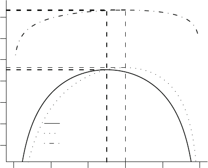
9.1 General Notions—Simple Cases 183

Here, the information is

I(P )=E{−∂

log L/∂P

}

= E{s/P

+(n − s)/(1 − P )

} (9.5)

= nP/P

+ n(1 − P )/(1 − P )

= n/[P (1 − P )].

We estimate the information by substituting the MLE of P into I(P ), yielding

I(p)=n/[p(1 − p)].

Figures

9.1, 9.2,and9.3 depict, r espectively, log L, U (P ), and I(P ), all

as a function of P . Three combinations of n and s were used in each graph.

These combinations correspond to p = .5,.6, and .6, respectively.

0.0 0.2 0.4 0.6 0.8 1.0

−140

−120

−100

−80

−60

−40

−20

Log Likelihood

s=50 n=100

s=60 n=100

s=12 n=20

Fig. 9.1 log likelihood functions for three one-sample binomial problems

In each case it can be seen that the value of P that makes the data most

likely to have occurred (the value that maximizes L or log L)isp given

above. Also, the score function (slope of log L) is zero at P = p.Notethat

the information function I(P ) is highest for P approaching 0 or 1 and is

lowest for P near .5, where there is maximum uncertainty about P .Note

also that while log L has the same shape for the s =60ands =12curves

in Figure

9.1, the range of log L is much greater for the larger sample size.

Figures

9.2 and 9.3 show that the larger sample size produces a sharper

likelihood. In other words, with larger n, one can zero in on the true value of

P with more precision.

184 9 Overview of Maximum Likelihood Estimation

0.0 0.2 0.4 0.6 0.8 1.0

−400

−200

200

400

600

Score

s=50 n=100

s=60 n=100

s=12 n=20

Fig. 9.2 Score functions (∂L/∂P)

0.0 0.2 0.4 0.6 0.8 1.0

200

400

600

800

1000

1200

Information

n=100

n=20

Fig. 9.3 Information functions (−∂

log L/∂P

)

In this binary response one-sample example let us now turn to inference

about the parameter P . First, we turn to the estimation of the variance of the

MLE, p. An estimate of this variance is given by the inverse of the information

at P = p:

9.2 Hypothesis Tests 185

Var(p)=I(p)

−1

= p(1 − p)/n. (9.6)

Note that the variance is smallest when the information is greatest (p =0

or 1).

The var iance estimate forms a basis for conﬁdence limits on the unknown

parameter. For large n,theMLEp is approximately normally distributed

with expected value (mean) P and variance P (1 − P )/n.Sincep(1 − p)isa

consistent estimate of P (1 − P )/n, it follows that p ± z[p(1 − p)/n]

1/2

is an

approximate 1 −α conﬁdence interval for P if z is the 1 − α/2criticalvalue

of the standard normal distribution.

9.2 Hypothesis Tests

Now let us turn to hypothesis tests about the unknown population parameter

P — H

: P = P

. There are three kinds of statistical tests that arise from

likelihood theory.

9.2.1 Likelihood Ratio Test

This test statistic is the ratio of the likelihood at the hypothesized parameter

values to the likelihood of the data at the maximum (i.e., at parameter values

= MLEs). It turns out that −2× the log of this likelihood ratio has desirable

statistical properties. The likelihood ratio test statistic is given by

LR = −2log(L at H

/L at MLEs)

= −2(log L at H

) − [−2(log L at MLEs)]. (9.7)

The LR statistic, for large enough samples, has approximately a χ

distribu-

tion with degrees of freedom equal to the number of parameters estimated, if

the null hypothesis is “simple,” that is, doesn’t involve any unknown param-

eters. Here LR has 1 d.f.

The value of log L at H

log L(H

)=s log(P

)+(n − s) log(1 − P

). (9.8)

The maximum value of log L (at MLE s) is

log L(P = p)=s log(p)+(n − s) log(1 − p). (9.9)

186 9 Overview of Maximum Likelihood Estimation

For the hypothesis H

: P = P

, the test statistic is

LR = −2{s log(P

/p)+(n − s) log[(1 − P

)/(1 − p)]}. (9.10)

Note that when p happens to equal P

, LR =0.Whenp is far from P

, LR will

be large. Suppose that P

=1/2, so that H

is P =1/2. For n = 100,s= 50,

LR =0.Forn = 100,s= 60,

LR = −2{60 log(.5/.6) + 40 log(.5/.4)} =4.03. (9.11)

For n =20,s= 12,

LR = −2{12 log(.5/.6) + 8 log(.5/.4)} = .81 = 4.03/5. (9.12)

Therefore, even though the best estimate of P is the same for these two cases,

the test statistic is mor e impressive when the sample size is ﬁve times larger.

9.2.2 Wald Test

The Wald test statistic is a g eneralization of a t-orz-statistic. It is a function

of the diﬀerence in the MLE and its hypothesized value, normalized by an

estimate of the standard deviation of the MLE. Here the statistic is

W =[p − P

]

/[p(1 − p)/n]. (9.13)

For large enough n, W is distributed as χ

with 1 d.f. For n = 100,s = 50,

W = 0. For the other samples, W is, respectively, 4.17 and 0.83 (note 0.83 =

4.17/5).

Many statistical packages treat

√

W as having a t distribution instead of

a normal distribution. As pointed out by Gould,

228

there is no basis for this

outside of ordinary linear models

9.2.3 Score Test

If the MLE happens to equal the hypothesized value P

, P

maximizes the

likelihood and so U (P

) = 0. Rao’s score statistic measures how far from zero

the sco re function is when evaluated at the null hypothesis. The score function

In linear regression, a t distribution is used to penalize for the fact that the variance

of Y |X is estimated. In models such as the logistic model, there is no separate vari-

ance parameter to estimate. Gould has done simulations that show that the normal

distribution provides more accurate P -values than the t for binary logistic regression.

9.2 Hypothesis Tests 187

(slope or ﬁrst derivative of log L) is normalized by the information (curvature

or second derivative o f −log L). The test statistic for o ur example is

S = U (P

)

/I(P

), (9.14)

which formally does not involve the MLE, p. The statistic can be simpliﬁed

as follows.

U(P

)=s/P

− (n − s)/(1 − P

)

I(P

)=s/P

+(n − s)/(1 − P

)

(9.15)

S =(s − nP

)

/[nP

(1 − P

)] = n(p − P

)

/[P

(1 − P

)].

Note that the numerator of S involves s − nP

, the diﬀerence between the

observed number of successes and the number of successes expected under H

As with the other two test statistics, S = 0 for the ﬁrst sample. For the

last two samples S is, respectively, 4 and .8 = 4/5. 1

9.2.4 Normal Distribution—One Sample

Suppose that a sample of size n is taken from a population for a random

variable Y that is known to be normally distributed with unknown mean

μ and variance σ

. Denote the observed values of the random variable by

,...,Y

. Now unlike the binary response case (Y = 0 or 1), we cannot

use the notion of the probability that Y equals an observed value. This is

because Y is continuous and the probability that it will take on a given value

is zero. We substitute the density function for the probability. The density

at a point y is the limit as d approaches zero of

Prob{y<Y ≤ y + d}/d =[F (y + d) − F (y)]/d, (9.16)

where F (y) is the normal cumulative distribution function (for a mean of μ

and variance of σ

). The limit of the r ight-hand side of the above equation as

d a pproaches zero is f (y), the density function of a normal distribution with

mean μ and variance σ

. This density function is

f(y)=(2πσ

)

−1/2

exp{−(y − μ)

/2σ

}. (9.17)

The likelihood of observing the observed sample values is the jo int density

of the Y s. The log likelihood function here is a function of two unknowns, μ

and σ

log L = −.5n log(2πσ

) − .5



i=1

− μ)

/σ

. (9.18)

188 9 Overview of Maximum Likelihood Estimation

It can be shown that the value of μ that maximizes log L is the value that min-

imizes the sum of squared deviations about μ, which is the sa mple mean

Y .

The MLE of σ



i=1

−

Y )

/n. (9.19)

Recall that the sample variance uses n −1 instead of n in the denominator. It

can be shown that the exp ected value of the MLE o f σ

, s

,is[(n −1)/n]σ

;

in other words, s

is too small by a factor of (n − 1)/n on the average. The

sample variance is unbiased, but b e ing unbiased does not necessar ily make

it a better estimator. The MLE has greater precision (smaller mean squared

error) in many cases.

9.3 General Case

Suppose we need to estimate a vector of unknown parameters B = {B

...,B

} from a sample of size n basedonobservationsY

,...,Y

.Denotethe

probability or density function of the random variable Y for the ith observa-

tion by f

(y; B). The likelihood for the i th observation is L

(B)=f

; B).

In the one-sample binary resp onse case, recall that L

(B)=L

(P )=

[1 − P ]

1−Y

. The likelihood function, or joint likelihood of the sample,

is given by

L(B)=



i=1

; B). (9.20)

The log likeliho od function is

log L(B)=



i=1

log L

(B). (9.21)

The MLE of B is that value of the vector B that maximizes log L(B)as

a function of B. In general, the solution for B requires iterative trial-and-

error methods as outlined later. Denote the MLE of B as b = {b

,...,b

The score vector is the vector of ﬁrst derivatives of log L(B) with respect to

,...,B

U(B)={∂/∂B

log L(B),...,∂/∂B

log L(B)}

=(∂/∂B)logL(B). (9.22)

The Fisher information matrix is the p × p matrix whose elements are the

negative of the expectation of all second partial derivatives of log L(B):

∗

(B)=−{E[(∂

log L(B)/∂B

∂B

)]}

p×p

= −E{(∂

/∂B∂B

′

)logL(B)}. (9.23)

9.3 General Case 189

The observed information matrix I(B)isI

∗

(B) without taking the expecta-

tion. In other words, observed values remain in the second derivatives:

I(B)=−(∂

/∂B∂B

′

)logL(B). (9.24)

This information matrix is often estimated from the sample using the es-

timated observed information I(b), by inserting b,theMLEofB,intothe

formula for I(B).

Under suitable conditions, which are satisﬁed for most situations likely

to be encountered, the MLE b for large samples is an optimal estimator

(has as great a chance of being close to the true parameter as all other

typ es of estimators) and has an approximate multivariate normal distribution

with mean vector B and variance–covariance matrix I

∗−1

(B), where C

−1

denotes the inverse of the matrix C.(C

−1

is the matrix such that C

−1

C is

the identity matrix, a matrix with ones on the diagonal and zeros elsewhere.

If C is a 1 × 1matrix,C

−1

=1/C.) A consistent estimator of the variance–

covariance matrix is given by the matrix V , obtained by inserting b for B in

I(B):V = I

−1

(b).

9.3.1 Global Test Statistics

Suppose we wish to test the null hypothesis H

: B = B

. The likelihood

ratio test statistic is

LR = −2log(L at H

/L at MLEs)

= −2[log L(B

) − log L(b)]. (9.25)

The corresponding Wald test statistic, using the estimated observed informa-

tion matrix, is

W =(b − B

)

′

I(b)(b − B

)=(b − B

)

′

−1

(b − B

). (9.26)

(A quadratic form a

′

Va is a matrix generalization of a

V .) Note that if the

number of estimated parameters is p =1,W reduces to (b −B

)

/V ,which

is the square of a z-ort-type s tatistic (estimate − hypothesized value divided

by estimated standa rd deviation of estimate).

The score statistic for H

S = U

′

−1

)U(B

). (9.27)

Note that as before, S does not requir e solving for the MLE. For large samples,

LR, W ,andS have a χ

distribution with p d.f. under suitable conditions.

190 9 Overview of Maximum Likelihood Estimation

9.3.2 Testing a Subset of the Parameters

Let B = {B

} and suppose that we wish to test H

: B

= B

.We

are treating B

as a nuisance parameter. For example, we may want to test

whether blood pressure and cholesterol are r isk factors after adjusting for

confounders age and sex. In that case B

is the pair of regression coeﬃcients

for bloo d pressure and cholesterol and B

is the pair of coeﬃcients for age

and sex. B

must be estimated to a llow adjustment for age and sex, although

is a nuisance parameter and is not of primary interest.

Let the number of parameters of interest be k so that B

is a vector of

length k. Let the number of “nuisance” or “adjustment” parameters be q,the

length of B

(note k + q = p).

Let b

∗

be the MLE of B

under the restriction that B

= B

. Then the

likelihood ratio statistic is

LR = −2[log L at H

− log L at MLE]. (9.28)

Now log L at H

is more complex than before because H

involves an unknown

nuisance parameter B

that must be estimated. log L at H

is the maximum

of the likelihood function for any value of B

but subject to the condition

that B

= B

.Thus

LR = −2[log L(B

∗

) − log L(b)], (9.29)

where as before b is the overall MLE of B.NotethatLR requires maximiz-

ing two log likelihood functions. The ﬁrst component of LR is a restricted

maximum likelihood and the second component is the overall or unrestricted

maximum.

LR is often computed by examining successively more complex models in

a stepwise fashion and calculating the increment in likelihood ratio χ

in the

overall model. The LR χ

for testing H

: B

=0whenB

is not in the

model is

LR(H

: B

=0|B

=0)=−2[log L(0, 0) − log L(0,b

∗

)]. (9.30)

Here we are specifying that B

is not in the model by setting B

= B

=0,

and we are testing H

: B

= 0. (We are also ignoring nuisance parameters

such as an intercept term in the test for B

=0.)

The LR χ

for testing H

: B

= B

= 0 is given by

LR(H

: B

= B

=0)=−2[log L(0, 0) − log L(b)]. (9.31)

Subtracting LR χ

for the smaller model from that of the larger model yields

−2[log L(0, 0) − log L(b)] −−2[log L(0, 0) − log L(0,b

2∗

)]

= −2[log L(0,b

∗

) − log L(b)], (9.32)

which is the same as above (letting B

=0).

9.3 General Case 191

Table 9.1 Example tests

Variables (Parameters) LR χ

Number of

in Model Parameters

Intercept, age 1000 2

Intercept, age, age

1010 3

Intercept, age, age

, sex 1013 4

For example, suppos e successively larger models yield the LR χ

sin

Table 9.1.TheLR χ

for testing for linearity in age (not adjusting for sex)

against quadratic alternatives is 1010 − 1000 = 10 with 1 d.f. The LR χ

for testing the added information provided by sex, adjusting for a quadratic

eﬀect of age, is 1013−1010 = 3 with 1 d.f. The LR χ

for testing the joint im-

portance of sex and the nonlinear (quadratic) eﬀect of age is 1013−1000 = 13

with 2 d.f.

To derive the Wald statistic for testing H

: B

= B

with B

being a

nuisance parameter, let the MLE b be partitioned into b = {b

}.Wecan

likewise partition the estimated variance–covariance matrix V into

V =



′



. (9.33)

The Wald statistic is

W =(b

− B

)

′

−1

− B

), (9.34)

which when k = 1 reduces to (estimate − hypothesized value)

/ estimated

variance, with the estimates adjusted for the parameters in B

The score statistic for testing H

: B

= B

does not require solving for

the full set of unknown parameters. Only the MLEs of B

must be computed,

under the restriction that B

= B

. This r estricted MLE is b

∗

from above.

Let U(B

∗

) denote the vector of ﬁrst derivatives of log L with respect to

all parameters in B, evaluated at the hypothesized parameter values B

for

the ﬁrst k parameters and at the restricted MLE b

∗

for the last q parameters.

(Since the last q estimates are MLEs, the la st q elements of U are zero, so

the formulas that follow simplify.) Let I(B

∗

) be the observed information

matrix evaluated at the same values of B as is U . The score statistic for

testing H

: B

= B

S = U

′

∗

−1

∗

)U(B

∗

). (9.35)

Under suitable conditions, the distribution of LR , W ,andS can b e ade-

quately approximated by a χ

distribution with k d.f. 2

192 9 Overview of Maximum Likelihood Estimation

9.3.3 Tests Based on Contrasts

Wald tests are also done by setting up a general linear contrast. H

: CB =0

is tested by a Wald statistic of the form

W =(Cb)

′

(CV C

′

)

−1

(Cb), (9.36)

where C is a contrast matrix that “picks oﬀ” the prop er elements of B.The

contrasts can be much more general by allowing elements of C to be other

than zero and one. For the normal linear model, W is converted to an F -

statistic by dividing by the rank r of C (normally the number of rows in

C), yielding a statistic with an F -distribution with r numerator degrees of

freedom.

Many interesting contrasts ar e tested by forming diﬀerences in predicted

values. B y forming more contrasts than are really needed, one can develop

a surprisingly ﬂexible approa ch to hypothesis testing using predicted values.

This has the major advantage of not requiring the analyst to account for how

the predictors are coded. Suppose that one wanted to assess the diﬀerence

in two vectors of predicted values, X

b − X

b =(X

− X

)b = Δb to test

: ΔB =0,whereΔ = X

−X

. The covariance matrix for Δb is given by

var(Δb)=ΔV Δ

′

. (9.37)

Let r be the rank of var(Δb), i.e., the number of non-linea rly-dependent

(non-redundant) diﬀerences of predicted values o f Δ. The value of r and the

rows of Δ that are not redundant may easily be determined using the QR

decomposition as done by the R function qr

.Theχ

statistic with r degrees

of freedom (or F -statistic upon dividing the statistic by r )maybeobtainedby

computing Δ

∗

′

where Δ

∗

is the subset of elements of Δ corresponding

to non-redundant contrasts and V

∗

is the corr e sponding sub-matrix of V .

The “diﬀerence in predictions” approach can be used to compare means

in a 30 year old male with a 40 year old fema le

. But the true utility of

the approach is most obvious when the contrast involves multiple nonlinear

terms for a single predictor, e.g., a spline function. To test for a diﬀerence

in two curves, one can compare predictions at one predictor value against

predictions at a series of values with at least one value that pertains to ea ch

basis function. Points can b e placed between every pair of knots and beyond

the outer knots, or just obtain predictions at 100 equally spaced X-values.

For example, in a 3-treatment comparison one could examine contrasts bet ween

treatments A and B, A and C, and B and C by obtaining predicted values for those

treatments, even though only two diﬀerences are required.

The rms command could be contrast(fit, list(sex=’male’,age=30),

list(sex=’female’,age=40)) where all other predictors are set to medians or

modes.

9.3 General Case 193

Suppose that there are three treatment groups (A, B, C) interacting with a

cubic spline function of X. If one wants to test the multiple degree of freedom

hypothesis that the proﬁle for X is the same for trea tment A and B vs. the

alternative hypothesis that there is a diﬀerence b etween A and B for at least

one value of X, one can compare predicted va lues at trea tment A and a vector

of X values against predicted values at treatment B and the same vector of

X values. If the X re lationship is linear, a ny two X values will suﬃce, and

if X is quadratic, a ny three points will suﬃce. It would be diﬃcult to test

complex hypotheses involving only 2 of 3 treatments using other methods.

The

contrast function in rms can estimate a wide variety of contrasts and

make joint tests involving them, automatically computing the number of non-

linearly-dep endent contrasts as the test’s degrees of freedom. See its help ﬁle

for several examples.

9.3.4 Which Test Statistics to Use When

At this point, one may ask why three types of test statistics are needed. The

answer lies in the statistica l properties of the three tests as well as in co m-

putational expense in diﬀer ent situations. From the standpoint of statistical

properties, LR is the best statistic, followed by S and W .Themajorsta-

tistical problem with W is that it is sensitive to pr oblems in the estimated

variance–covariance matrix in the full mo del. For some models, most notably

the logistic regression model,

278

the variance–covariance estimates can be too

large as the eﬀects in the model become very strong, resulting in values o f

W that are too small (or signiﬁcance levels that are to o large). W is also

sensitive to the way the parameter appears in the model. For example, a test

of H

: log odds ratio = 0 will yield a diﬀer ent value of W than will H

odds ratio = 1.

Relative computational eﬃciency of the three types of tests is also an issue.

Computation of LR and W requires estimating all p unknown parameters,

and in addition LR re quires re-estimating the last q parameters under that

restriction that the ﬁrst k parameters = B

. Therefore, when one is contem-

plating whether a set of parameters should be added to a model, the score

test is the easiest test to carry out. For example, if one were interested in

testing all two-way interactions among 4 predictors, the score test statistic

for H

: “no interactions present” could be computed without estimating the

4 ×3/2 = 6 interaction eﬀects. S would a lso be appealing for testing linearity

of eﬀects in a model—the nonlinear spline terms could be tested for signiﬁ-

cance after adjusting for the linear eﬀects (with estimation of only the linear

eﬀects). Only parameters for linear eﬀects must be estimated to compute

S, resulting in fewer numerical problems such as lack of convergence of the

Newton–Raphson algorithm.

194 9 Overview of Maximum Likelihood Estimation

Table 9.2 Choice of test statistics

Type of Test Recommended Test Statistic

Global association LR (S for large no. parameters)

Partial association W (LR or S if problem with W)

Lack of ﬁt, 1 d.f. W or S

Lack of ﬁt, > 1d.f. S

Inclusion of additional predictors S

The Wald tests are very easy to make after all the parameters in a model

have been estimated. Wald tests are thus appealing in a multiple regression

setup when one wants to test whether a given predictor or set of predic-

tors is “signiﬁcant.” A score test would require re-estimating the regression

coeﬃcients under the restr iction that the parameters of interest equal zero.

Likelihood ratio tests are used often for testing the global hypothesis that

no eﬀects are signiﬁcant, as the log likelihood evaluated at the MLEs is al-

ready available from ﬁtting the model and the log likelihood evaluated at

a “null model” (e.g., a model containing only an intercept) is often easy to

compute. Likelihood ratio tests should also be used when the validity of a

Wa ld test is in question as in the example cited above.

Table

9.2 summarizes recommendations for choice of test statistics for

various situations.

9.3.5 Example: Binomial—Comparing Two

Proportions

Suppose that a binary random variable Y

represents responses for population

1andY

represents responses for population 2. Let P

=Prob{Y

=1}

and assume that a random sample has b een drawn from each population

with respective sample sizes n

and n

. The sample values are denoted by

,...,Y

,i= 1 or 2. Let



j=1



j=1

, (9.38)

the resp ective observed number of “successes” in the two samples. Let us test

the null hypothesis H

: P

= P

based on the two samples.

The likelihood function is

L =



i=1



j=1

(1 − P

)

1−Y

9.4 Iterative ML Estimation 195



i=1

(1 − P

)

−s

(9.39)

log L =



i=1

log(P

)+(n

− s

) log(1 − P

)}. (9.40)

Under H

= P

= P ,so

log L(H

)=s log(P )+(n − s) log(1 − P ), (9.41)

where s = s

+ s

,n = n

+ n

. The (restricted) MLE of this common P is

p = s/n and log L at this value is s log(p)+(n − s)log(1− p).

Since the original unrestricted log likelihood function contains two terms

with separate parameters, the two parts may be maximized separately giving

MLEs

= s

and p

= s

. (9.42)

log L evaluated at these (unrestricted) MLEs is

log L = s

log(p

)+(n

− s

)log(1− p

)

+ s

log(p

)+(n

− s

)log(1− p

). (9.43)

The likelihood ratio statistic for testing H

: P

= P

is then

LR = −2{s log(p)+(n − s) log(1 − p)

− [s

log(p

)+(n

− s

) log(1 − p

) (9.44)

+ s

log(p

)+(n

− s

) log(1 − p

)]}.

This statistic for large enough n

and n

has a χ

distribution with 1 d.f.

since the null hypothesis involves the estimation of one fewer parameter than

does the unrestricted case. This LR statistic is the likelihood ratio χ

statistic

for a 2 × 2 contingency table. It can be shown that the correspo nding score

statistic is equivalent to the Pearson χ

statistic. The better LR statistic can

be used routinely over the Pearson χ

for testing hypotheses in contingency

tables.

9.4 Iterative ML Estimation

In most cases, one cannot explicitly solve for MLEs but must use trial-and-

error numerical metho ds to solve for parameter values B that maximize

log L(B) or yield a score vector U(B) = 0. One of the fastest and most ap-

plicable methods for maximizing a function is the Newton–Raphson method,

which is based on approximating U (B) by a linear function of B in a small

196 9 Overview of Maximum Likelihood Estimation

region. A starting estimate b

of the MLE b is made. The linear approximation

(a ﬁrst-order Taylor series approximation)

U(b)=U (b

) − I(b

)(b − b

) (9.45)

is equated to 0 and solved by b yielding

b = b

+ I

−1

)U(b

). (9.46)

The pro cess is continued in like fashion. At the ith step the next estimate is

obtained from the previous estimate using the formula

i+1

= b

+ I

−1

)U(b

). (9.47)

If the log likelihood actually worsened at b

i+1

, “step halving” is used; b

i+1

is replaced with (b

+ b

i+1

)/2. Further step halving is done if the log like-

lihood still is worse than the log likelihood at b

, after which the original

iterative strategy is resumed. The Newton–Raphson iterations continue until

the −2 log likelihood changes by only a small amount over the previous iter-

ation (say .025). The reasoning behind this stopping rule is that estimates of

B that change the − 2 log likelihood by less than this amount do not aﬀect

statistical inference since −2 log likelihood is on the χ

scale.3

9.5 Robust Estimation of the Covariance Matrix

The estimator for the covariance matrix of b found in Section

9.3 assumes that

the model is correctly speciﬁed in terms of distribution, regression assump-

tions, and independence assumptions. The model may be incorrect in a va-

riety of ways such as non-independence (e.g., repeated measurements within

subjects), lack o f ﬁt (e.g., omitted covariable, incorrect covariable transfor-

mation, omitted interaction), and distributional (e.g., Y has a Γ distribution

instead of a normal distribution). Variances and covariances, and hence con-

ﬁdence intervals and Wald tests, will b e incorrect when these assumptions

are viola ted.

For the case in which the observations a re independent and identically

distributed but other assumptions are possibly violated, Huber

312

provided

a covariance matrix estimator that is consistent. His “sandwich” estimator is

given by

H = I

−1

(b)[



i=1

′

−1

(b), (9.48)

where I(b) is the observed information matrix (Equation

9.24)andU

is the

vector of deriva tives, with respect to all parameters, of the log likelihood

component for the ith observation (assuming the log likelihoo d can be par-

titioned into per-observation contributions). For the normal multiple linear

regression case, H was derived by White:

659

9.5 Robust Estimation of the Covariance Matrix 197

′

−1

[



i=1

− X

′

](X

′

−1

, (9.49)

where X is the design matrix (including an intercept if appropriate) and X

is the vector of predictors (including an intercept) for the i th observation.

This covariance estimator allows for any pattern of variances of Y |X across

observations. Note that even though H improves the bias of the covariance 4

matrix of b, it may actually have larger mean squared error than the ordinary

estimate in some cases due to increased variance.

164, 529

When observations are dependent within clusters, and the number of ob-

servations within clusters is very small in comparison to the total sample

size, a simple adjustment to Equation 9.48 canbeusedtoderiveappro-

priate covariance matrix estimates (see Lin [

407, p. 2237], Rogers,

529

and

Lee et al. [393, E q. 5.1, p. 246]). One merely accumulates sums of elements of

U within clusters before computing cross-product terms:

= I

−1

(b)[



i=1

{(



j=1

)(



j=1

)

′

}]I

−1

(b), (9.50)

where c is the number of clusters, n

is the number of observations in the ith

cluster, U

is the contribution of the jth observation within the ith cluster to

the score vector, and I(b) is computed as before ignoring clusters. For a model

such as the Cox model which has no per-observation sco re contributions,

special score residuals

393, 407, 410, 605

are used for U.

Bootstrapping can also be used to derive ro bust covar iance matrix esti-

mates

177, 178

in many cases, especially if covariances of b that are not condi-

tional on X are appropriate. One merely generates approximately 200 samples

with replacement from the original dataset, computes 200 sets of parameter

estimates, and computes the sample covariance matrix of these parameter es-

timates. Sampling with replacement from entire clusters can be used to derive

variance estimates in the presence of intracluster correlation.

188

Bo otstrap 5

estimates of the conditional variance–covariance matrix given X are harder

to obtain and depend on the model assumptions being satisﬁed. The simpler

unconditional estimates may b e more appropriate for many non-experimental

studies where one may desire to “penalize” for the X being random variables.

It is interesting that these unconditional estimates may be very diﬃcult to ob-

tain parametrically, since a multivariate distribution may need to be assumed

for X.

The previous discussion addresses the use of a “working independence

model” with clustered data. Here one estimates regression coeﬃcients assum-

ing independence of all records (observations). Then a sandwich or bootstrap

method is used to increase standard erro rs to reﬂect some re dundancy in the

correlated observations. The parameter estimates will often be consistent es-

timates of the true parameter values, but they may be ineﬃcient for certain

cluster or correlation structures.

198 9 Overview of Maximum Likelihood Estimation

The rms package’s robcov function computes the Huber robust covariance

matrix estimator, and the bootcov function computes the bootstrap covariance

estimator. Both of these functions allow for clustering.

9.6 Wald, Score, and Likelihood-Based Conﬁdence

Intervals

A1− α conﬁdence interval for a parameter β

is the set of all values β

that if hypothesized would be accepted in a test of H

: β

= β

at the

α level. What test should form the ba sis for the conﬁdence interva l? The

Wa ld test is most frequently used because of its simplicity. A two-sided 1 −α

conﬁdence interval is b

±z

1−α/2

s,wherez is the critical value from the normal

distribution and s is the estimated standard error of the parameter estimate

The pr oblem with s discussed in Section 9.3.4 pointsoutthatWald

statistics may not always be a g ood basis. Wald-ba sed conﬁdence intervals are

also symmetric even though the coverage probability may not be.

160

Score-

and LR-based conﬁdence limits have deﬁnite advantages. When Wald-type7

conﬁdence intervals are appropriate, the ana lyst may consider insertion of

robust covariance estimates (Section 9.5) into the conﬁdence interval fo rmulas

(note that adjustments for heterogeneity and correlated observations are not

available for score and LR statistics).

Wald– (asymptotic normality) based statistics are convenient for deriving

conﬁdence intervals for linear or more complex combinations of the model’s

parameters. As in Equation

9.36, the va riance–covariance matrix of Cb,where

C is an appropriate matrix and b is the vector of parameter estimates, is

CV C

′

,whereV is the variance matrix of b. In regression models we commonly

substitute a vector of predictors (and optional inter cept) for C to obtain the

variance of the linear predictor Xb as

var(Xb)=XVX

′

. (9.51)

See Section

9.3.3 for related information.

This is the basis for conﬁdence limits computed by the R rms package’s Predict,

summary,andcontrast functions. When the robcov function has been used to replace

the information-matrix-based covariance matrix with a Huber robust covariance esti-

mate with an optional cluster sampling correction, the functions are using a “robust”

Wald statistic basis. When the bootcov function has been used to replace the model

ﬁt’s covariance matrix with a bootstrap unconditional covariance matrix estimate,

the two functions are computing conﬁdence limits based on a normal distribution but

using more nonparametric covariance estimates.

9.7 Bootstrap Conﬁdence Regions 199

9.6.1 Simultaneous Wald Conﬁdence Regions

The conﬁdence intervals just discussed are pointwise conﬁdence intervals.

For OLS regression there are methods for computing conﬁdence intervals

with exact simultaneous conﬁdence coverage for multiple estimates

374

.There

are approximate methods for simultaneous conﬁdence limits for all models

for which the vector of estimates b is approximately multiva riately normally

distributed. The method of Hothorn et al.

307

is quite general; in their R

package multcomp’s glht function, the user can specify any contrast matrix over

which the individual conﬁdence limits will be simultaneous. A special case

of a contrast matrix is the design matrix X itself, resulting in simultaneous

conﬁdence bands for any number of predicted values. An example is shown

in Figure

9.5. See Section 9.3.3 for a good use for simultaneous contrasts.

9.7 Bootstrap Conﬁdence Regions

A more nonparametric method for computing conﬁdence intervals for func-

tions of the vector of parameters B can be based on bootstrap percentile

conﬁdence limits. For each s ample with replacement from the origina l dataset,

one computes the MLE of B, b, and then the quantity of interest g(b). Then

the gs are sorted and the desired quantiles are computed. At least 1000 bo ot-

strap samples will be needed for accur ate a ssessment of outer conﬁdence

limits. This method is suitable for obtaining pointwise conﬁdence bands for

a nonlinear regression function, say, the relationship between age and the log

o dds of disease. At each of 100 age values the predicted logits are computed

for each bo otstrap sample. Then separately for each age point the 0.025 and

0.975 quantiles of 1000 estimates of the logit are computed to derive a 0.95

conﬁdence band. Other more complex bootstrap schemes will achieve some-

what greater accuracy of conﬁdence interval coverage,

178

and as described

in Section

9.5 one can use variations on the basic b ootstrap in which the

predictors are considered ﬁxed and/or cluster sampling is taken into account.

The

R function bootcov in the rms package bootstraps model ﬁts to obtain

unconditional (with respect to predictors) bootstrap distributions with or

without cluster sampling. bootcov stores the matrix of bootstrap regression

coeﬃcients so that the bootstrapped quantities of interest can be computed

in one sweep of the coeﬃcient matrix once bootstrapping is completed. 9

For many regression models. the rms package’s Predict, summary,and

contrast functions make it easy to compute pointwise bootstrap conﬁdence

intervals in a variety of contexts. As an example, consider 200 simulated

x values from a lo g-normal distribution and simulate binary y from a true

population binary logistic model given by

200 9 Overview of Maximum Likelihood Estimation

Prob(Y =1|X = x)=

1+exp[−(1 + x/2)]

. (9.52)

Not knowing the true model, a quadratic logistic model is ﬁtted. The

R code

needed to generate the data and ﬁt the model is given below.

require(rms)

n ← 200

set.seed(15)

x1 ← rnorm (n)

logit ← x1/2

y ← ifelse (runif(n) ≤ plogis(logit), 1, 0)

dd ← datadist(x1); options(datadist= ' dd ' )

f ← lrm(y ∼ pol(x1,2), x=TRUE , y=TRUE)

print(f, latex =TRUE)

Logistic Regression Model

lrm(formula = y ~ pol(x1, 2), x = TRUE, y = TRUE)

Model Likelihood Discrimination Rank Discrim.

Ratio Test Indexes Indexes

Obs 200 LR χ

16.37 R

0.105 C 0.642

097d.f. 2 g 0.680 D

0.285

1 103 Pr(>χ

) 0.0003 g

1.973 γ 0.286

max |

∂ log L

∂β

| 3×10

−9

0.156 τ

0.143

Brier 0.231

Coef S.E. Wald Z Pr(> |Z|)

Intercept -0.0842 0.1823 -0.46 0.6441

x1 0.5902 0.1580 3.74 0.0002

0.1557 0.1136 1.37 0.1708

latex(anova(f), file= '', table.env=FALSE )

d.f. P

x1 13.99 2 0.0009

Nonlinear 1.88 1 0.1708

TOTAL 13.99 2 0.0009

The bootcov function is used to draw 1000 resamples to obtain bootstrap

estimates of the covariance matrix of the regression coeﬃcients as well as

to save the 1000 × 3 matrix of regression coeﬃcients. Then, because indi-

vidual regression coeﬃcients for x do not tell us much, we summarize the

9.7 Bootstrap Conﬁdence Regions 201

x-eﬀect by computing the eﬀect (on the logit scale) of increasing x from 1

to 5. We ﬁrst compute bootstrap nonparametric percentile conﬁdence inter-

vals the long way. The 1000 bootstrap estimates of the log odds ratio are

computed easily using a single matrix multiplication with the diﬀerence in

predictions approach, multiplying the diﬀerence in two design matrices, and

we obtain the bootstrap estimate of the standard error of the log odds ratio

by computing the sample standard deviation of the 1000 values

. Bootstrap

pe rcentile conﬁdence limits are just sample quantiles from the bootstrapped

log odds ratios.

# Get 2-row design matrix for obtaining predicted values

# for x = 1 and 5

X ← cbind (Intercept=1,

predict(f, data.frame (x1=c(1,5)), type= ' x ' ))

Xdif ← X[2,,drop=FALSE] - X[1,,drop=FALSE ]

Xdif

Intercept pol(x1, 2)x1 pol(x1, 2)x1

∧

20 4 24

b ← bootcov(f, B=1000)

boot.log.odds.ratio ← b$boot.Coef %*% t(Xdif)

sd(boot.log.odds.ratio )

[1] 2.752103

# This is the same as from summary(b, x=c(1,5)) as summary

# uses the bootstrap covariance matrix

summary(b, x1=c(1,5))[1, ' S.E. ' ]

[1] 2.752103

# Compare this s.d. with one from information matrix

summary(f, x1=c(1,5))[1, ' S.E. ' ]

[1] 2.988373

# Compute percentiles of bootstrap odds ratio

exp(quantile(boot.log.odds.ratio , c(.025 , .975 )))

2.5% 97.5%

2.795032 e+00 2.067146 e+05

# Automatic:

summary(b, x1=c(1,5))[ ' Odds Ratio ' ,]

As indicated below, this standard deviation can also be obtained by using the

summary function on the object returned by bootcov,asbootcov returns a ﬁt object

like one from lrm except with the bootstrap covariance matrix substituted for the

information-based one.

202 9 Overview of Maximum Likelihood Estimation

Low High Diff. Effect S.E.

1.000000 e+00 5.000000 e+00 4.000000 e+00 4.443932e+02 NA

Lower 0.95 Upper 0.95 Type

2.795032 e+00 2.067146 e+05 2.000000 e+00

print(contrast(b, list(x1=5), list(x1=1), fun=exp))

Contrast S.E. Lower Upper Z Pr(>|z|)

11 6.09671 2.752103 1.027843 12.23909 2.22 0.0267

Confidence intervals are 0.95 bootstrap nonparametric percentile intervals

# Figure 9.4

hist(boot.log.odds.ratio , nclass =100, xlab= ' log(OR) ' ,

main= '')

log(OR)

Frequency

0 5 10 15

Fig. 9.4 Distribution of 1000 bootstrap x=1:5 log odds ratios

Figure

9.4 shows the distribution of log odds ratio s.

Now consider conﬁdence bands for the true log odds that y =1,across

a sequence of x values. The Predict functio n automatically calculates point-

by-point bootstrap percentiles, basic bo otstrap, or BCa

203

conﬁdence limits

when the ﬁt has passed through bootcov. Simultaneous Wald-based conﬁ-

dence intervals

307

and Wald intervals substituting the bootstrap covariance

matrix estimator are added to the plot when Predict calls the multcomp pack-

age (Figure

9.5).

x1s ← seq(0, 5, length =100)

pwald ← Predict(f, x1=x1s)

psand ← Predict(robcov (f), x1=x1s)

pbootcov ← Predict(b, x1=x1s , usebootcoef =FALSE)

pbootnp ← Predict(b, x1=x1s)

pbootbca ← Predict(b, x1=x1s , boot.type= ' bca ' )

pbootbas ← Predict(b, x1=x1s , boot.type= ' basic ' )

psimult ← Predict(b, x1=x1s, conf.type= ' simultaneous ' )

9.8 Further Use of the Log Likelihood 203

z ← rbind ( ' Boot percentile ' = pbootnp ,

' Robust sandwich ' = psand ,

' Boot BCa ' = pbootbca ,

' Boot covariance+Wald ' = pbootcov ,

Wald = pwald ,

' Boot basic ' = pbootbas ,

Simultaneous = psimult)

z$class ← ifelse (z$.set. %in% c( ' Boot percentile ' , ' Boot bca ' ,

' Boot basic ' ), ' Other ' , ' Wald ' )

ggplot (z, groups =c( ' .set. ' , ' class ' ),

conf= ' line ' , ylim=c(-1, 9), legend.label =FALSE)

See Problems at chapter’s end for a worrisome investigation o f bootstrap con-

ﬁdence interval coverage using simulation. It appears that when the model’s

log odds distribution is not symmetric and includes very high or very low

probabilities, neither the bootstrap percentile nor the bootstrap BCa inter-

vals have good coverage, while the basic bootstrap and ordinary Wald in-

tervals are fairly accurate

. It is diﬃcult in general to know when to trust

the bootstrap for logistic and perhaps other models when computing conﬁ-

dence intervals, and the simulation problem suggests that the basic bootstrap

should be used more frequently. Similarly, the distribution of bootstrap eﬀect

estimates can be suspect. Asymmetry in this distribution does not imply that

the true sampling distribution is asymmetric or that the percentile intervals

are preferred.

9.8 Further Use of the Log Likelihood

9.8.1 Rating Two M odels, Penalizing for Complexity

Suppose that from a single sample two competing models were develop ed. Let

the r espective −2 log likelihoods for these models be denoted by L

and L

and let p

and p

denote the number of para meters estimated in each model.

Suppose that L

. It may be tempting to rate model one as the “best”

ﬁtting or “best” predicting model. That model may provide a better ﬁt for

the data at hand, but if it required many more parameters to be estimated,

it may not be better “for the money.” If both models were applied to a new

sample, model one’s overﬁtting of the original dataset may actually result in

a worse ﬁt on the new dataset.

Limited simulations using the conditional bootstrap and Firth’s penalized likeli-

hood

281

did not show signiﬁcant improvement in conﬁdence interval coverage.

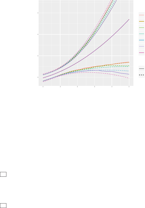
204 9 Overview of Maximum Likelihood Estimation

0.0

2.5

5.0

7.5

012345

log odds

.set.

Boot percentile

Robust sandwich

Boot BCa

Boot covariance+Wald

Wald

Boot basic

Simultaneous

Other

Wald

Fig. 9.5 Predicted log odds and conﬁdence bands for seven types of conﬁdence in-

tervals. Seven categories are ordered top to bottom corresponding to order of low er

conﬁdence bands at x1=5. Dotted lines are for Wald–t ype methods that yield sym-

metric conﬁdence intervals and assume normality of point estimators.

Akaike’s information criterion (AIC

33, 359, 633

)providesamethodforpe-

nalizing the log likelihood achieved by a given model for its complexity to

obtain a more unbiased assessment o f the model’s worth. The penalty is

to subtract the number of parameters estimated from the log likelihood, or

equivalently to add twice the number of parameters to the −2 log likeliho od.

The penalized log likelihood is analogous to Mallows’ C

in ordinary multiple

regression. AIC would choose the model by comparing L

+2p

to L

+2p

and picking the model with the lower value. We often use AIC in “adjusted10

”form:

AIC = LR χ

− 2p. (9.53)

Breiman [

66, Section 1.3] and Chatﬁeld [100, Section 4] discuss the fallacy of

AIC and C

for selecting from a series of non-prespeciﬁed models.11

9.8.2 Testing Whether One Model Is Better

than Another

One way to test whether one model (A) is better than another (B)isto

embedbothmodelsinamoregeneralmodel(A + B). Then a LR χ

test

9.8 Further Use of the Log Likelihood 205

can be done to test whether A is better than B by changing the hypothesis

to test whether A adds predictive information to B (H

: A + B>B)and

whether B adds information to A (H

: A + B>A). The approach of testing

A>Bvia testing A+ B>Band A +B>Ais especially useful for selecting

from competing predictors such as a multivaria ble model and a subjective

assessor.

131, 264, 395, 669

Note that LR χ

for H

: A + B>Bminus LR χ

for H

: A + B>A

equals LR χ

for H

: A has no predictive information minus LR χ

for

: B has no predictive information,

665

the diﬀerence in LR χ

for testing

each model (set of variables) separately. This gives further support to the use

of two separately computed Akaike’s information criteria for rating the two

sets of variables.

See Section 9.8.4 for an example.

9.8.3 Unitless Index of Predictive Ability

The global likelihood ratio test for regression is useful for determining whether

any predictor is associated with the resp onse. If the sample is large enough,

even weak associations can b e “statistically signiﬁcant.” Even though a like-

lihood ratio test does not shed light on a model’s predictive strength, the log

likelihood (L.L.) can still be useful here. Consider the following L.L.s:

Best (lowest) possible −2 L.L.:

∗

= −2 L.L. for a hypothetical model that pe rfectly predicts the outcome.

−2 L.L. achieved:

L = −2 L.L. for the ﬁtted model.

Worst −2 L.L.:

= −2 L.L. for a model that has no predictive information.

The last −2 L.L., for a “no information” model, is the −2 L.L. under the null

hypothesis that all regression coeﬃcients except for intercepts are zero. A “no

information” model often contains only an intercept and some distributional

parameters (a variance, for example). 13

The quantity L

− L is LR, the log likelihood ratio statistic for testing

the global null hypothesis that no predicto rs are related to the response. It

is also the −2 log likelihood “explained” by the model. The best (lowest) −2

L.L. is L

∗

, so the amount of L.L. that is capable of being explained by the

model is L

−L

∗

. The fraction of −2 L.L. explained that was capable of being

explained is

− L)/(L

− L

∗

)=LR/(L

− L

∗

). (9.54)

206 9 Overview of Maximum Likelihood Estimation

The fraction of log likelihood explained is analogous to R

in an ordinary

linear model, although Korn and Simon

365, 366

provide a much more precise

notion.

Akaike’s information criterion can be used to penalize this measure of

asso ciation for the number of parameters estimated (p, say) to transform

this unitless measure of association into a quantity that is analogous to the

adjusted R

or Mallows’ C

in ordinary linear regression. We let R denote

the squa re root of such a penalized fraction of log likelihood explained. R is

deﬁned by

=(LR − 2p)/(L

− L

∗

). (9.55)

The R index can be used to assess how well the model compares with a

“perfect” model, as well as to judge whether a more complex model has pre-

dictive strength that justiﬁes its additional parameters. Had p been used in

Equation

9.55 rather than 2p, R

is negative if the log likelihood explained

is less than what one would expect by chance. R will be the square root of

1 − 2p/ (L

− L

∗

) if the model p erfectly predicts the response. This upper

limit will be near one if the sample size is large.

Partial R indexes can also be deﬁned by substituting the −2 L.L. explained

for a given factor in place of that for the entire model, LR. The “penalty

factor” p becomes one. This index R

partial

is deﬁned by

partial

=(LR

partial

− 2)/(L

− L

∗

), (9.56)

which is the (penalized) fraction of −2 log likelihood explained by the pre-

dictor. Here LR

partial

is the log likelihood ratio statistic for testing whether

the predictor is associated with the response, after adjustment for the other

predictors. Since such likelihood ratio statistics are tedious to compute, the

1 d.f. Wald χ

can be substituted for the LR statistic (keeping in mind that

diﬃculties with the Wald statistic can arise).

Liu and Dyer

424

and Cox and Wermuth

136

point out diﬃculties with the

measure for binary logistic models. Cox and Snell

135

and Magee

432

used

other analogies to derive other R

measures that may have better properties.

For a sample of size n and a Wald statistic for testing overall association,

they deﬁned

n + W

=1− exp(−LR/n) (9.57)

=1− λ

2/n

where λ is the null model likelihood divided by the ﬁtted model likelihood. I n

the case of ordinary least squares with normality b oth of the above indexes

are equal to the traditional R

. R

is equivalent to Maddala’s index [

431,

Eq. 2.44]. Cragg and Uhler

137

and Nagelkerke

471

suggested dividing R

9.8 Further Use of the Log Likelihood 207

its maximum attainable value

max

=1− exp(−L

/n) (9.58)

to derive R

which ranges from 0 to 1. This is the form of the R

index we

use throughout.

For penalizing for overﬁtting, see Verweij and van Houwelingen

640

for an

overﬁtting-corrected R

that uses a cross-validated likelihood. 14

9.8.4 Unitless Index of Adequacy of a Subset

of Predictors

Log likelihoods are also useful for quantifying the predictive information con-

tained in a subset of the predictors compared with the information contained

in the entire set of predictors.

264

Let LR again denote the −2 log likelihood

ratio statistic for testing the joint signiﬁcance of the full set of predictors. Let

denote the −2 log likelihood ratio statistic for testing the importance of

the subset of predictors of interest, excluding the other predictors from the

model. A measure of adequacy of the subset for predicting the response is

given by

A = LR

/LR. (9.59)

A is then the proportion o f log likelihood explained by the subset with refer-

ence to the log likelihood explained by the entire set. When A = 1 , the subset

contains a l l the predictive information found in the whole set of predictors;

that is, the subset is adequate by itself and the additional predictors contain

no independent information. When A = 0, the subset contains no predictive

information by itself.

Caliﬀ et al.

used the A index to quantify the adequacy (with respect to

prognosis) of two competing sets of predictors that each describe the extent of

coronary artery disea se. The response variable was time until ca rdiovascular

death and the statistical model used was the Cox

132

proportional hazards

model. Some of their results are repr oduced in Table

9.3. A chance-corrected 15

adequacy measure could be derived by squaring the ratio of the R-index for

the subset to the R-index for the whole set. A formal test of superiority of

= maximum % stenosis over X

= jeopardy score can be obtained by

testing whether X

adds to X

(LR χ

=57.5 − 42.6=14.9) and whether

adds to X

(LR χ

=57.5 −51.8=5.7). X

adds more to X

(14.9) than

adds to X

(5.7). The diﬀerence 14.9 − 5.7=9.2 equals the diﬀerence in

single factor χ

(51.8 − 42.6)

665

208 9 Overview of Maximum Likelihood Estimation

Table 9.3 Completing prognostic markers

Predictors Used LR χ

Adequacy

Coronary jeopardy score 42.6 0.74

Maximum % stenosis in each artery 51.8 0 .90

Combined 57.5 1.00

9.9 Weighted Maximum Likelihood Estimation

It is commonly the case that data elements represent combinations of values

that pertain to a set of individuals. This occurs, fo r example, when unique

combinations of X and Y are determined from a massive dataset, along with

the frequency of occurrence of each combination, for the purpo se of reducing

the size of the dataset to analyze. For the ith combination we have a case

weight w

that is a positive integer representing a frequency. Assuming that

observations represented by combination i are independent, the likelihood

needed to represent all w

observations is computed simply by multiplying

all of the likelihood elements (each having value L

), yielding a total likeli-

hood contribution for combination i of L

or a log likelihood contribution

of w

log L

. To obtain a likelihood for the entire dataset one computes the

product over all combinations. The total log likelihood is



log L

.Asan

example, the weighted likelihood that would be used to ﬁt a weighted logistic

regression model is given by

L =



i=1

(1 − P

)

(1−Y

)

, (9.60)

where there a re n combinations,



i=1

>n,andP

is Prob[Y

=1|X

]as

dictated by the model. Note that in general the correct likelihood function

cannot be obtained by weighting the data and using an unweighted likelihood.

By a small leap one can obtain weighted maximum likelihood estimates

from the above method even if the weights do not represent frequencies or

even integers, as long as the weights are no n-negative. Non-frequency weights

are commonly used in sample surveys to adjust estimates back to better

represent a target population when some types of subjects have been over-

sampled from that population. Analysts should beware of possible losses in

eﬃciency when obtaining weighted estimates in sample surveys.

363, 364

Mak-

ing the regression estimates conditional on sampling strata by including strata

as covariables may be preferable to re-weighting the strata. If weighted esti-

mates must be obtained, the weighted likelihood function is generally valid

for obtaining properly weighted parameter estimates. However, the variance–

covariance matrix obtained by inverting the information matrix from the

weighted likelihood will not be c orrect in general. For one thing, the sum of

the weights may be far from the number of subjects in the sample. A rough

9.10 Penalized Maximum Lik elihood Estimation 209

approximation to the variance–covariance matrix may be obtained by ﬁrst

multiplying each weight by n/



and then computing the weighted in-

formation matrix, where n is the number of actual subjects in the sample.

9.10 Penalized Maximum Likelihood Estimation

Maximizing the log likelihood provides the best ﬁt to the dataset at hand,

but this can also result in ﬁtting no ise in the data. For example, a categor-

ical predictor with 20 levels can produce extreme estimates for so me of the

19 regression parameters, especially for the small cells (see Section

4.5). A

shrinkage approach will often result in regression coeﬃcient estimates that

while biased are lower in mean squared error and hence are more likely to be

close to the true unknown parameter values. Ridge regression is one approach

to shrinkage, but a more general and better developed approach is penalized

maximum likelihood estimation,

237, 388, 639, 641

which is r eally a special case 17

of Bayesian modeling with a Gaussian prior. Letting L denote the usual like-

lihoo d function and λ be a penalty factor, we maximize the penalized log

likelihood given by

log L −



i=1

)

, (9.61)

where s

,...,s

are scale factors chosen to make s

unitless. Most au-

thors standardize the data ﬁrst and do not have scale factors in the equation,

but Equation

9.61 has the advantage of allowing estimation of β on the orig-

inal scale of the data. The usual methods (e.g., Newton–Raphson) ar e used

to maximize

9.61.

The choice o f the scaling constants has received far too little attention in

the ridge regression and p enalized MLE literature. It is common to use the

standard deviation of each column of the design matrix to scale the corre-

sponding parameter. For models containing nothing but continuous varia bles

that enter the regr ession linearly, this is usually a reasonable approach. For

continuous variables represented with multiple terms (one of which is lin-

ear), it is not always reasonable to scale each nonlinear term with its own

standard deviation. For dummy variables, scaling using the standard devia-

tion (



d(1 − d), where d is the mean of the dummy variable, i.e., the frac-

tion of observations in that cell) is problematic since this will result in high

prevalance cells getting more shrinkage than low prevalence ones because the

high prevalence cells will dominate the penalty function.

An advantage of the formulation in Equation

9.61 is that one can assign

scale constants of zero for parameters for which no shrinkage is desired.

237, 639

For example, one may have prior beliefs that a linear additive model will ﬁt

the data. In that case, nonlinear and non-additive terms may be penalized.

210 9 Overview of Maximum Likelihood Estimation

For a categorical predictor having c levels, users of ridge regression often do

not recognize that the amount of shrinkage and the predicted values from the

ﬁtted model depend on how the design matrix is coded. For example, one will

get diﬀerent predictions depending on which cell is chosen as the reference

cell when constructing dummy variables. The setup in Equatio n

9.61 has the

same problem. For example, if for a three-category factor we use category 1

as the reference cell and have parameters β

and β

, the unscaled penalty

function is β

+ β

. If category 3 were used as the reference cell instead, the

pe nalty would b e β

+(β

− β

)

. To get around this pr oblem, Verweij and

van Houwelingen

639

proposed using the penalty function



(β

−β)

,where

β is the mean of all cβs. This causes shrinkage of all parameters toward

the mean parameter value. Letting the ﬁrst category be the reference cell,

we use c − 1 dummy variables and deﬁne β

≡ 0. For the case c =3the

sum o f squares is 2[β

+ β

− β

]/3. For c =2thepenaltyisβ

/2. If no

scale constant is used, this is the same as scaling β

with

√

2 × the standard

deviation of a binary dummy variable with prevalance of 0.5.

The sum of squares can be written in matrix form as [β

,...,β

]

′

(A − B)[β

,...,β

], where A is a c − 1 × c − 1identitymatrixandB is

a c − 1 × c − 1 matrix all of whose elements are

.19

For general penalty functions such as that just described, the penalized

log likelihood can be generalized to

log L −

λβ

′

Pβ. (9.62)

For purposes of using the Newton–Raphson procedure, the ﬁrst derivative

of the penalty function with respect to β is −λP β, and the nega tive of the

second derivative is λP .

Another problem in penalized estimation is how the choice of λ is made.20

Many authors use cross-validation. A limited number of simulatio n stud-

ies in binary logistic regression modeling has shown that for each λ being

considered, at least 10-fold cross-validation must b e done so a s to obtain a

reasonable estimate of predictive accuracy. Even then, a smoother

207

(“ su-

per s moother”) must be used on the (λ, accuracy) pairs to allow location of

the optimum value unless one is careful in choosing the initial sub-samples

and uses these same splits thro ughout. Simulation studies have shown that a

modiﬁed AIC is not only much quicker to compute (since it requires no cross-

validation) but performs better at ﬁnding a good value of λ (see below).21

For a given λ, the eﬀective number of parameters being estimated is re-

duced because of shrinkage. Gray [237, Eq. 2.9] and others estimate the ef-

fective degrees of freedom by computing the expected value of a global Wa ld

statistic for testing association, when the null hyp othesis of no association is

true. The d.f. is equal to

trace[I(

)V (

)], (9.63)

9.10 Penalized Maximum Lik elihood Estimation 211

where

is the p enalized MLE (the parameters that maximize Equa-

tion

9.61), I is the information matrix computed from ignoring the penalty

function, and V is the covariance matrix computed by inverting the infor-

mation matrix that included the second derivatives with respect to β in the

penalty function. 22

Gray [237, Eq. 2.6] states that a better estimate of the variance–covariance

matrix for

than V (

)is

∗

= V (

)I(

)V (

). (9.64)

Therneau (personal communication, 2000) has found in a limited number

of simulation studies that V

∗

underestimates the true variances, and that a

be tter estimate of the variance–covariance matrix is simply V (

), assuming

that the model is correctly speciﬁed. This is the covariance matrix used by

default in the rms package (the user can request that the sandwich estimator

be used instead) and is in fact the one Gray used for Wald tests.

Penalization will bias estimates of β, so hypothesis tests and co nﬁdence

intervals using

may not have a simple interpretation. The same prob-

lem arises in sco re and likelihood ratio tests. So far, penalization is better

understood in pure predictio n mode unless Bayesian methods are used.

Equation

9.63 can be used to derive a modiﬁed AIC (see [639,Eq.6]

and [

641, Eq. 7]) on the model χ

scale:

LR χ

− 2 × eﬀective d.f., (9.65)

where LR χ

is the likelihood ratio χ

for the penalized model, but ignoring

the penalty function. If a variety of λ are tried and one plots the (λ,AIC)

pairs, the λ that maximizes AIC will often be a good choice, that is, it is

likely to be near the value of λ that maximizes predictive accuracy on a

future dataset

Note that if o ne does penalized maximum likelihood estimation where a set

of variables being penalized has a negative value for the unp enalized χ

−2 ×

d.f., the value of λ that will optimize the overall model AIC will be ∞.

As an example, consider some simulated data (n = 100) with one predictor

in which the true model is Y = X

+ ǫ,whereǫ has a standard normal

distribution and so does X

. We use a series of penalties (found by trial a nd

error) that give rise to sensible eﬀective d.f., and ﬁt penalized restricted cubic

spline functions with ﬁve knots. We penalize two ways: all terms in the model

including the coeﬃcient of X

, which in reality needs no p enalty; and only

the nonlinear terms. The following R program, in conjunction with the rms

package, does the job.

Several examples from simulated datasets have shown that using BIC to cho ose a

penalty results in far too much shrinkage.

212 9 Overview of Maximum Likelihood Estimation

set.seed(191)

x1 ← rnorm (100)

y ← x1 + rnorm (100)

pens ← df ← aic ← c(0,.07,.5,2,6,15,60)

all ← nl ← list()

for(penalize in 1:2) {

for(i in 1:length (pens )) {

f ← ols(y ∼ rcs(x1,5), penalty=

list(simple =if(penalize ==1) pens[i] else 0,

nonlinear=pens[i]))

df[i] ← f$stats[ ' d.f. ' ]

aic[i] ← AIC(f)

nam ← paste (if(penalize == 1) ' all ' else ' nl ' ,

' penalty: ' , pens[i], sep= '')

nam ← as.character (pens[i])

p ← Predict(f, x1=seq(-2.5 , 2.5, length =100),

conf.int=FALSE )

if(penalize == 1) all[[nam]] ← p else nl[[nam]] ← p

}

print(rbind(df=df, aic=aic))

}

[,1] [,2] [,3] [,4] [,5] [,6]

df 4.0000 3.213591 2.706069 2.30273 2.029282 1.822758

aic 270.6653 269.154045 268.222855 267.56594 267.288988 267.552915

[,7]

df 1.513609

aic 270.805033

[,1] [,2] [,3] [,4] [,5] [,6]

df 4.0000 3.219149 2.728126 2.344807 2.109741 1.960863

aic 270.6653 269.167108 268.287933 267.718681 267.441197 267.347475

[,7]

df 1.684421

aic 267.892073

all ← do.call( ' rbind ' , all); all$type ← ' Penalize All '

nl ← do.call( ' rbind ' , nl) ; nl$type ← ' Penalize Nonlinear '

both ← as.data.frame(rbind.data.frame(all, nl))

both$Penalty ← both$.set.

ggplot(both, aes(x=x1, y=yhat, color=Penalty )) + geom_line () +

geom_abline (col=gray(.7)) + facet_grid (∼ type)

# Figure 9.6

The left panel in Figure 9.6 corresponds to penalty = list(simple=a, nonlin-

ear=a) in the R program, meaning that all parameters except the intercept are

shrunk by the same amount a (this would be more appropriate had there been

multiple predictors). As eﬀective d.f. get smaller (penalty factor gets larger),

the regression ﬁts get ﬂatter (too ﬂat for the largest p enalties) and conﬁdence

bands get narrower. The right graph corresponds to penalty=list(simple=0,

nonlinear=a), causing only the cubic spline terms that are nonlinear in X

to be shrunk. As the amount of shrinkage increases (d.f. lowered), the ﬁts

become more linear and closer to the true regression line (longer dotted line).

Again, conﬁdence intervals become smaller.23

9.11 Further Reading 213

Penalize All Penalize Nonlinear

−2

−2 −1 0 1 2 −2 −1 0 1 2

yhat

Penalty

0.07

0.5

Fig. 9.6 Penalized least squares estimates for an unnecessary ﬁve-knot restricted

cubic spline function. In the left graph all parameters (except the intercept) are

penalized. The eﬀective d.f. are 4, 3.21, 2.71, 2.30, 2.03, 1.82, and 1.51. In the right

graph, only parameters associated with nonlinear functions of X

are penalized. The

eﬀective d.f. are 4, 3.22, 2.73, 2.34, 2.11, 1.96, and 1.68.

9.11 Further Reading

Boos

has some nice generalizations of the score test. Morgan et al.

464

show

how score test χ

statistics may negative unless the expected information matrix

is used.

See Marubini and Valsecchi [444, pp. 164–169] for an excellent description of

the relationship between the three types of test statistics.

References [115,507] have good descriptions of methods used to maximize log L.

As Long and Ervin

426

argue, for small sample sizes, the usual Huber–White co-

variance estimator should not be used because there the residuals do not have

constant variance even under homoscedasticity. They showed that a simple cor-

rection due to Efron and others can result in substantially better estimates.

Lin and Wei,

410

Binder,

and Lin

407

have applied the Huber estimator to the

Cox

132

survival model. Freedman

206

questioned the use of sandwich estima-

tors because they are often used to obtain the right v a riances on the wrong

parameters when the model doesn’t ﬁt. He also has some excellent background

information.

Feng et al.

188

showed that in the case of cluster correlations arising from re-

peated measurement data with Gaussian errors, the cluster bootstrap performs

excellently even when the num ber of observations per cluster is large and the

number of subjects is small. Xiao and Abrahamowicz

676

compared the cluster

bootstrap with a tw o-stage cluster bootstrap in the context of the Cox model.

214 9 Overview of Maximum Likelihood Estimation

Graubard and Korn

235

and Fitzmaurice

195

describe the kinds of situations in

which the working independence model can be trusted.

Minkin,

460

Alho,

Doganaksoy and Schmee,

160

and Meeker and Escobar

452

discuss the need for LR and score-based conﬁdence intervals. Alho found that

score-based intervals are usually more tedious to compute, and provided use-

ful algorithms for the computation of either type of interval (see also [

452]

and [

444, p. 167]). Score and LR intervals require iterative computations and

have to deal with the fact that when one parameter is changed (e.g., b

is re-

stricted to be zero), all other parameter estimates change. DiCiccio and Efron

157

provide a method for very accurate conﬁdence intervals for exponential families

that requires a modest amount of additional computation. Venzon and Mo ol-

gavkar provide an eﬃcient general method for computing LR-based intervals.

636

Brazzale and Davison

developed some promising and feasible ways to make

unconditional likelihood-based inferences more accurate in small samples.

Carpenter and Bithell

have an excellent overview of several variations on the

bootstrap for obtaining conﬁdence limits.

Tibshirani and Knight

610

developed an easy to program approach for deriving

simultaneous conﬁdence s ets that is likely to be useful for getting simultaneous

conﬁdence regions for the entire vector of model parameters, for population val-

ues for an entire sequence of predictor values, and for a set of regression eﬀects

(e.g., interquartile-range odds ratios for age for both sexes). The basic idea is

that during the, say, 1000 bootstrap repetitions one stores the −2 log likelihood

for each model ﬁt, being careful to compute the likelihood at the current bo ot-

strap parameter estimates but with respect to the original data matrix, not

the bootstrap sample of the data matrix. To obtain an approximate simultane-

ous 0.95 conﬁdence set one computes the 0.95 quantile of the −2 log likelihoo d

values and determines whic h vectors of parameter estimates correspond to −2

log likelihoods that are at least as small as the 0.95 quantile of all −2 log like-

lihoo d s. Once the q ualifying parameter estimates are found, the q uantities of

interest are computed from those parameter estimates and an outer envelope

of those quantities is found. Computations are facilitated with the rms pack age

confplot function.

van Houwelingen and le Cessie [633, Eq. 52] showed, consistent with AIC, that

the average optimism in a mean logarithmic (minus log likelihood) quality score

for logistic mo dels is p/n.

Schwarz

560

derived a diﬀerent penalty using large-sample Bayesian prop erties

of competing models. His Bay esian Information Criterion (BIC) chooses the

model having the lowest value of L +1/2p log n or the highest value of LR

− p log n. Kass and Raftery have done several studies of BIC.

337

Smith

and Spiegelhalter

576

and Laud and Ibrahim

377

discussed other useful gener-

alizations of likelihood p enalties. Zheng and Loh

685

studied several penalty

measures, and found that AIC does not penalize enough for overﬁtting in the

ordinary regression case. Kass and Raftery [

337, p. 790] provide a nice review

of this topic, stating that “AIC picks the correct model asymptotically if the

complexity of the true model grows with sample size” and that “AIC selects

models that are too big even when the sample size is large.” But they also cite

other papers that show the existence of cases where AIC can work b etter than

BIC. According to Buckland et al.,

BIC “assumes that a true mo del exists

and is low-dimensional.”

Hurvich and Tsai

314, 315

made an improvemen t in AIC that resulted in m uch

better model selection for small n. They deﬁned the corrected AIC as

AIC

=LRχ

− 2p[1 +

p +1

n − p − 1

]. (9.66)

9.11 Further Reading 215

In [

314] they contrast asymptotically eﬃcient model selection with AIC when

the true model has inﬁnitely many parameters with improvements using other

indexes such as AIC

when the model is ﬁnite.

One diﬃculty in applying the Schwarz, AIC

, and related criteria is that with

censored or binary responses it is not clear that the actual sample size n should

b e used in the formula.

Goldstein,

222

Willan et al.,

669

and Royston and Thompson

534

have nice dis-

cussions on comparing non-nested regression models. Schemper’s method

549

useful for testing whether a set of v ariables provides signiﬁcantly greater infor-

mation (using an R

measure) than another set of variables.

van Houwelingen and le Cessie [633, Eq. 22] recommended using L/2 (also called

the Kullback–Leibler error rate) as a quality index.

Schemper

549

provides a bootstrap technique for testing for signiﬁcant diﬀer-

ences between correlated R

measures. Mittlb

ock and Schemper,

461

Schemper

and Stare,

554

Korn and Simon,

365, 366

Menard,

454

and Zheng and Agresti

684

have excellent discussions ab out the pros and cons of various indexes of the

predictive value of a model.

Al-Radi et al.

presented another analysis comparing competing predictors

using the adequacy index and a receive r operating characteristic curv e area

approach based on a test for whether one predictor has a higher probability of

being “more concordant” than another.

[55, 97, 409] provide good variance–covariance estimators from a weighted max-

imum likelihood analysis.

Huang and Harrington

310

develop ed penalized partial likelihood estimates for

Cox models and provided useful background information and theoretical results

about improvements in mean squared errors of regression estimates. They used

a bootstrap error estimate for selection of the penalty parameter.

Sardy

538

proposes that the square roots of the diagonals of the in verse of the

covariance matrix for the predictors b e used for scaling rather than the standard

deviations.

Park and Hastie

483

and articles referenced therein describe how quadratic pe-

nalized logistic regression automatically sets coeﬃcient estimates for empty cells

to zero and forces the sum of k coeﬃcients for a k-level categorical predictor to

equal zero.

Greenland

241

has a nice discussion of the relationship between penalized max-

imum likelihood estimation and mixed eﬀects models. He cautions against esti-

mating the shrinkage parameter.

See

310

forabootstrapapproachtoselectionofλ.

Verweij and van Houwelingen [639, Eq. 4] derived another expression for d.f., but

it requires more computation and did not perform any better than Equation

9.63

in choosing λ in several examples tested.

See v an Houwelingen and Thorogood

631

for an approximate empirical Bayes

approach to shrinkage. See Tibshirani

608

for the use of a non-smooth penalty

function that results in variable selection as well as shrinkage (see Section

4.3).

Verweij and v a n Houwelingen

640

used a “cross-validated likelihood” based on

leave-out-one estimates to penalize for ov erﬁtting. Wang and Taylor

652

pre-

sented some methods for carrying out hypothesis tests and computing con-

ﬁdence limits under penalization. Moons et al.

462

presented a case study of

penalized estimation and discussed the advantages of penalization.

216 9 Overview of Maximum Likelihood Estimation

Table 9.4 Likelihood ratio global test statistics

Variables in Mo del LR χ

age 100

sex 108

age, sex 111

age

age, age

102

age, age

, sex 115

9.12 Problems

1. A sample of size 100 from a normal distribution with unknown mean and

standard deviation (μ and σ) yielded the following log likelihood values

when computed at two values of μ.

log L(μ =10,σ =5)=−800

log L(μ =20,σ =5)=−820.

What do you know about μ? What do you know about

Y ?

2. Several regression models were considered for predicting a response. LR χ

(corrected for the intercept) for models containing various combinations of

variables are found in Table

9.4. Compute all possible meaningful LR χ

For each, state the d.f. and an approximate P -value. State which LR χ

involving only one variable is not very meaningful.

3. For each problem below, rank Wald, score, and LR statistics by overall

statistical properties and then by computational convenience.

a. A forward stepwise variable selection (to be later accounted for with the

bootstrap) is desired to determine a concise model that contains most

of the independent information in all potential predictors.

b. A test of indep endent association of each variable in a given model (each

variable adjusted for the eﬀects of all other variables in the given model)

is to be obtained.

c. A model that contains only additive eﬀects is ﬁtted. A large number

of potential interaction terms are to be tested using a global (multiple

d.f.) test.

4. Consider a univariate saturated model in 3 treatments (A, B, C) that is

quadratic in age. Write out the model with all the βs, and write in detail

the contrast for comparing treatment B with treatment C for 30 year olds.

Sketch out the same contrast using the “diﬀerence in predictions” approach

without simpliﬁcation.

9.12 Problems 217

5. Simulate a binary logistic model for n = 300 with an average fraction of

events somewhere between 0.15 and 0.3. Use 5 continuous covariates and

assume the model is everywhere linear. Fit an unpenalized model, then

solve for the optimum quadratic penalty λ. Relate the resulting eﬀective

d.f. to the 15:1 rule of thumb, and compute the heuristic shrinkage coeﬃ-

cient ˆγ for the unpenalized model and for the optimally penalized model,

inserting the eﬀective d.f. for the number of non-intercept parameters in

the model.

6. For a similar s etup as the binary logistic model simulation in Section

9.7,

do a Monte Car l o simulation to determine the coverage probabilities for

ordinar y Wald and for three types of bootstr ap conﬁdence intervals for the

true x=5 to x=1 log odds ratio. In addition, consider the Wald-type con-

ﬁdence interval arising from the sandwich covariance estimator. Estimate

the non-coverage probabilities in both tails. Use a sample size n = 200

with the single predictor x

having a standard lo g-normal distribution,

and the true model being logit(Y =1)=1+x

/2. Determine whether

increasing the sample size r elieves any problem you observed. Some R code

for this simulation is on the web site.

Chapter 10

Binary Logistic Regression

10.1 Model

Binary responses are commonly studied in many ﬁelds. Examples include 1

the presence or absence of a particular disease, death during surgery, or a

consumer purchasing a product. Often one wishes to study how a set of

predictor variables X is related to a dichotomous response variable Y .The

predictors may describe such quantities as treatment assignment, dosage, risk

factors, and calendar time.

For convenience we deﬁne the response to be Y = 0 or 1, with Y =1

denoting the occurrence of the event of interest. Often a dichotomous outcome

can be studied by calculating certain proportions, for example, the prop ortion

of deaths among females and the prop ortion among males. However, in many

situations, there are multiple descriptors , or one or mor e of the descriptors

are continuous. Without a statistical model, studying patterns such as the

relationship between age and occurrence of a disease, for example, would

require the creation of arbitrary age groups to allow estimation of disease

prevalence as a function of age.

Letting X denote the vector of pr edictors {X

,...,X

}, a ﬁrst attempt

at modeling the response might use the ordinary linear regression model

E{Y |X} = Xβ, (10.1)

since the expectation of a binary variable Y is Prob{Y =1}. However, such

a model by deﬁnition cannot ﬁt the data over the whole range of the pre-

dictors since a purely linear model E{Y |X} =Prob{Y =1|X} = Xβ can

allow Prob{Y =1} to exceed 1 or fall below 0. The statistical model that is

generally preferred for the analysis of binary responses is instead the binary

logistic regression model, stated in terms of the probability tha t Y =1given

X, the values of the predictors:

F.E. Harrell, Jr., Regression Modeling Strategies, Springer Series

in Statistics, DOI 10.1007/978-3-319-19425-7

219

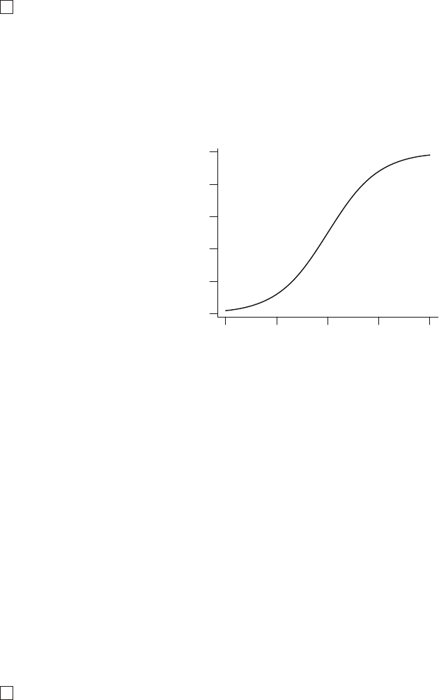
220 10 Binary Logistic Regression

Prob{Y =1|X} =[1+exp(−Xβ)]

−1

. (10.2)

As before, Xβ stands for β

+ β

+ ...+ β

. The binary lo-

gistic regression mo del was developed primarily by Cox

129

and Walker and

Duncan.

647

The regression parameters β are estimated by the method of2

maximum likelihood (see be low).

The function

P =[1+exp(−x)]

−1

(10.3)

is called the logistic function. This function is plotted in Figure

10.1 for x

varying from −4 to +4. This function has an unlimited range for x while P

is restricted to range from 0 to 1.

−4 −2 0 2 4

0.0

0.2

0.4

0.6

0.8

1.0

Fig. 10.1 Logistic function

For future derivations it is useful to express x in terms o f P .Solvingthe

equation above for x by using

1 − P =exp(−x)/[1+exp(−x)] (10.4)

yields the inverse of the logistic function:

x = log[P/(1 − P )] = log[odds that Y = 1 occurs] = logit{Y =1}. (10.5)

Other methods that have been used to analyze binary response data in-

clude the probit model, which writes P in terms of the cumulative normal

distribution, and discriminant ana lysis. Probit regression, although assuming

a similar shape to the logistic function for the regression relationship be-

tween Xβ and Prob{Y =1}, involves more cumbersome calculations, and

there is no natural interpretation of its regression parameters. In the past,

discriminant analysis has been the predominant method since it is the sim-

plest computationally. However, it makes more assumptions than logistic re-

gression. The model used in discr iminant a nalysis is stated in terms of the3

10.1 Model 221

distribution of X given the outcome group Y , even though one is seldom in-

terested in the distribution of the predictors per se. The discriminant model

has to be inverted using Bayes’ rule to derive the quantity of primary in-

terest, Prob{Y =1}. By contrast, the logistic model is a direct probability

model since it is stated in terms of Prob{Y =1|X}. Since the distribution

of a binary random variable Y is completely deﬁned by the true probability

that Y = 1 and since the model makes no assumption about the distribu-

tion of the predictors, the logistic model makes no distributional assumptions

whatso ever.

10.1.1 Model Assumptions and Interpretation

of Parameters

Since the logistic model is a dir ect probability model, its only assumptions

relate to the form of the regression equation. Regression assumptions are

veriﬁable, unlike the assumption of multivariate normality made by discrimi-

nant analysis. The logistic model assumptions are most easily understood by

transforming Prob{Y =1} to make a model that is linear in Xβ:

logit{Y =1|X} = logit(P) = log[P/(1 − P )]

= Xβ, (10.6)

where P =Prob{Y =1|X}. Thus the model is a linear regression model in

the log odds that Y = 1 since logit(P )isaweightedsumoftheXs. If all

eﬀects are additive (i.e., no interactions a re present), the model assumes that

for every predictor X

logit{Y =1|X} = β

+ β

+ ...+ β

= β

+ C, (10.7)

where if all other factors are held constant, C is a constant given by

C = β

+ β

+ ...+ β

j−1

+ β

j+1

+ ...+ β

. (10.8)

The parameter β

is then the change in the log odds per unit change in

if X

represents a single factor that is linear and does no t interact with

other factors and if all other factors are held constant. Instead of writing this

relationship in terms of log odds, it could just as easily be written in terms

of the odds that Y =1:

odds{Y =1|X} =exp(Xβ), (10.9)

222 10 Binary Logistic Regression

and if all factors other than X

are held constant,

odds{Y =1|X} =exp(β

+ C)=exp(β

)exp(C). (10.10)

The regression parameters can also be written in terms of odds r atios.The

odds that Y =1whenX

is increased by d, divided by the odds at X

odds{Y =1|X

,...,X

+ d,...,X

}

odds{Y =1|X

,...,X

}

exp[β

+ d)] exp(C)

[exp(β

)exp(C)]

(10.11)

=exp[β

+ β

d − β

]=exp(β

d).

Thus the eﬀect of increasing X

by d is to increase the odds that Y =1by

afactorofexp(β

d), or to increase the log odds that Y = 1 by an increment

of β

d. In general, the ra tio of the odds of response for an individual with

predictor variable values X

∗

compared with an individua l with predictors

X is

∗

: X odds ratio = exp(X

∗

β)/ exp(Xβ)

=exp[(X

∗

− X)β]. (10.12)

Now consider some special cases of the logistic multiple regression model.

If there is only one predictor X and that predictor is binary, the model can

be written

logit{Y =1|X =0} = β

logit{Y =1|X =1} = β

+ β

. (10.13)

Here β

is the log odds of Y =1whenX = 0. By subtracting the two

equations above, it can be seen that β

is the diﬀerence in the log odds

when X = 1 as compared with X = 0, which is equivalent to the log of the

ratio of the odds when X = 1 compared with the odds when X =0.The

quantity exp(β

) is the odds ratio for X = 1 compared with X = 0. Letting

=Prob{Y =1|X =0} and P

=Prob{Y =1|X =1}, the regression

parameters are interpreted by

= logit(P

) = log[P

/(1 − P

)]

= logit(P

) − logit(P

) (10.14)

=log[P

/(1 − P

)] − log[P

/(1 − P

)]

=log{[P

/(1 − P

)]/[P

/(1 − P

)]}.

10.1 Model 223

Since there are only two quantities to model and two free para meters,

there is no way that this two-sample model can’t ﬁt; the model in this case

is essentially ﬁtting two cell proportions. Similarly, if there are g −1 dummy

indicator Xs representing g groups, the ANOVA-type log istic model must

always ﬁt.

If there is one co ntinuous predictor X, the model is

logit{Y =1|X} = β

+ β

X, (10.15)

and without further modiﬁcation (e.g., taking log transformation of the pre-

dictor), the model assumes a straight line in the log odds, or that an increase

in X by one unit increases the odds by a facto r of exp(β

Now consider the simplest analysis of covariance model in which there are

two treatments (indicated by X

= 0 or 1) and one continuous covariable

). The simplest logistic model for this setup is

logit{Y =1|X} = β

+ β

, (10.16)

which can be written also as

logit{Y =1|X

=0,X

} = β

+ β

logit{Y =1|X

=1,X

} = β

+ β

. (10.17)

The X

=1:X

= 0 odds ratio is exp(β

), independent of X

. The odds

ratio for a one-unit increase in X

is exp(β

), independent of X

This model, with no term for a possible interaction between treatment

and covariable, assumes that for each treatment the relationship between X

and log odds is linear, and that the lines have equal slope; tha t is, they are

parallel. Assuming linearity in X

, the only way that this model can fail is

for the two slopes to diﬀer. Thus, the only assumptions that need veriﬁcation

are linearity and lack of interaction b etween X

and X

To adapt the model to allow or test for interaction, we write

logit{Y =1|X} = β

+ β

, (10.18)

where the derived va riable X

is deﬁned to be X

.Thetestforlackof

interaction (equal slopes) is H

: β

= 0. The model can b e ampliﬁed as

logit{Y =1|X

=0,X

} = β

+ β

logit{Y =1|X

=1,X

} = β

+ β

(10.19)

= β

′

+ β

′

224 10 Binary Logistic Regression

Table 10.1 Eﬀect of an odds ratio of two on various risks

Without Risk Factor With Risk Factor

Probability Odds Odds Probability

.2 .25 .5 .33

.5 1 2.67

.8 4

8.89

.9 9 18 .95

.98 49

98 .99

where β

′

= β

+ β

and β

′

= β

+ β

. The model with interaction is therefore

equivalent to ﬁtting two separate logistic models with X

as the only predic-

tor, one model for each treatment group. Here the X

=1:X

= 0 odds

ratio is exp( β

+ β

10.1.2 Odds Ratio, Risk Ratio, and Risk Diﬀerence

As discussed above, the logistic model quantiﬁes the eﬀect of a predictor in

terms of an odds ratio or log odds ratio. An odds ratio is a na tural descrip-

tion of an eﬀect in a probability model since an odds ratio can be constant.

For example, suppose that a given risk factor doubles the odds of disease.

Table

10.1 shows the eﬀect of the r isk factor for various levels of initial risk.

Since odds have an unlimited range, any pos itive odds ratio will still yield

a valid pr obability. If one attempted to describe an eﬀect by a risk ratio, the

eﬀect can only occur over a limited range of risk (probability). For example, a

risk ratio of 2 can only apply to risks below .5; above that point the risk ratio

must diminish. (Risk ratios are similar to odds ratios if the risk is small.)

Risk diﬀerences have the same diﬃculty; the risk diﬀerence cannot be con-

stant and must depend on the initial risk. Odds ratios, on the other hand, can

describe an eﬀect over the entire range of risk. An odds ratio can, for example,

describe the eﬀect of a treatment indep endently of covariables aﬀecting risk.

Figure

10.2 depicts the relationship between risk of a subject without the risk

factor and the increase in risk for a variety of relative increases (odds ratios).

It demonstrates how absolute risk increase is a function of the baseline r isk.

Risk increase will also be a function of factors that interact with the risk fac-

tor, that is, factors that modify its relative eﬀect. Once a model is developed

for estimating Prob{Y =1|X}, this model can easily be used to estimate the

absolute risk increase as a function of baseline risk factors as well as inter-

acting factors. Let X

be a binary risk factor and let A = {X

,...,X

} be

the other factors (which for convenience we assume do not intera c t with X

Then the estimate of Prob{Y =1|X

=1,A}−Prob{Y =1|X

=0,A} is

10.1 Model 225

0.0 0.2 0.4 0.6 0.8 1.0

0.0

0.1

0.2

0.3

0.4

0.5

0.6

Risk for Subject Without Risk Factor

Increase in Risk

1.1

1.25

1.5

1.75

Fig. 10.2 Absolute beneﬁt as a function of risk of the event in a control subject and

the relative eﬀect (odds ratio) of the risk factor. The odds ratios are given for each

curve.

Table 10.2 Example binary response data

Females Age : 37 39 39 42 47 48 48 52 53 55 56 57 58 58 60 64 65 68 68 70

Response:

00000010000001001111

Males Age: 34 38 40 40 41 43 43 43 44 46 47 48 48 50 50 52 55 60 61 61

Response:

11000111001110111111

1+exp−[

+ ...+

]

−

1+exp−[

+ ...+

]

(10.20)

1+(

1−

)exp(−

)

−

where

R is the estimate of the baseline risk, Prob{Y =1|X

=0}.Therisk

diﬀerence estimate can be plotted against

R or against levels of variables in A

to display absolute risk increase against overall risk (Figure

10.2) or against

speciﬁc subject characteristics. 4

10.1.3 Detailed Example

Consider the data in Table

10.2. A graph of the data, along with a ﬁtted

logistic model (described later), appears in Figure

10.3. The graph also dis-

plays proportions of responses obtained by stratifying the data by sex and

226 10 Binary Logistic Regression

age group (< 45, 45 − 54, ≥ 55). The age p oints on the a bscissa for these

groups are the overall mean ages in the three age intervals (40.2, 49.1, and

61.1, respectively).

require(rms)

getHdata (sex.age.response)

d ← sex.age.response

dd ← datadist (d); options (datadist = ' dd ' )

f ← lrm(response ∼ sex + age, data=d)

fasr ← f # Save for later

w ← function (...)

with(d, {

m ← sex== ' male '

f ← sex== ' female '

lpoints(age[f], response [f], pch=1)

lpoints(age[m], response [m], pch=2)

af ← cut2(age , c(45,55), levels.mean =TRUE)

prop ← tapply(response , list(af, sex), mean ,

na.rm=TRUE)

agem ← as.numeric (row.names (prop))

lpoints(agem, prop[, ' female ' ],

pch=4, cex=1.3, col= ' green ' )

lpoints(agem, prop[, ' male ' ],

pch=5, cex=1.3, col= ' green ' )

x ← rep (62, 4); y ← seq(.25, .1, length=4)

lpoints(x, y, pch=c(1, 2, 4, 5),

col=rep(c( ' blue ' , ' green ' ),each=2))

ltext(x+5, y,

c( ' F Observed ' , ' M Observed ' ,

' F Proportion ' , ' M Proportion ' ), cex=.8)

}) # Figure 10.3

plot(Predict(f, age=seq(34, 70, length=200), sex , fun=plogis),

ylab= ' Pr[response ] ' , ylim=c(-.02 , 1.02), addpanel =w)

ltx ← function (fit) latex(fit, inline=TRUE , columns =54,

file= '', after= ' $. ' , digits=3,

size= ' Ssize ' , before= ' $X\\hat{\\beta}= ' )

ltx(f)

β = −9.84 + 3.49[male] + 0.158 age.

Descriptive statistics for assessing the association between sex and re-

sponse, age group and response, and age group and response stratiﬁed by

sex are found below. Corresponding ﬁtted logistic models, with sex coded as

0 = female, 1 = male are also given. Mo dels were ﬁtted ﬁrst with sex as the

only predictor, then with age as the (continuous) predictor, then with sex and

age simultaneously. Fir st consider the relationship between sex and response,

ignoring the eﬀect of age.

10.1 Model 227

age

Pr[response]

0.2

0.4

0.6

0.8

40 50 60 70

F Observed

M Observed

F Proportion

M Proportion

female

male

Fig. 10.3 Data, subgroup proportions, and ﬁtted logistic model, with 0.95 pointwise

conﬁdence bands

sex response

Frequency

Row Pct 0 1 Total Odds/Log

F 14 6 20 6/14=.429

70.00 30.00 -.847

M 6 14 20 14/6=2.33

30.00 70.00 .847

Total 20 20 40

M:F odds ratio = (14/6)/(6/14) = 5.44, log=1.695

Statistics for sex × response

Statistic d.f. Value P

1 6.400 0.011

Likelihood Ratio χ

1 6.583 0.010

Parameter Estimate Std Err Wald χ

−0.8473 0.4880 3.0152

1.6946 0.6901 6.0305 0.0141

228 10 Binary Logistic Regression

Note that the estimate of β

is the log odds for females and that

is the

log odds (M:F) ratio.

= .847, the log o dds for males. The likelihood

ratio test for H

: no eﬀect of sex on proba bility of response is obtained as

follows.

Log likeliho od (β

=0):−27.727

Log likelihood (max) : −24.435

LR χ

: β

=0) :−2(−27.727 −−24.435) = 6.584.

(Note the agreement of the LR χ

with the contingency table likelihood ratio

, and compare 6.584 with the Wald statistic 6.03.)

Next, consider the relationship between age and response, ignoring sex.

age response

Frequency

Row Pct 0 1 Total Odds/Log

<45 8 5 13 5/8=.625

61.5 38.4 -.47

45-54 6 6 12 6/6=1

50.0 50.0 0

55+ 6 9 15 9/6=1.5

40.0 60.0 .405

Total 20 20 40

55+ : <45 odds ratio = (9/6)/(5/8) = 2.4, log=.875

Parameter Estimate Std Err Wald χ

−2.7338 1.8375 2.2134 0.1368

0.0540 0.0358 2.2763 0.1314

The estimate of β

is in rough agr eement with that obtained from the

frequency table. The 55+ : < 45 log odds ratio is .875, and since the respective

mean ages in the 55+ and <45 age groups are 61.1 and 40.2, an estimate of

the log odds ratio increase per year is .875/(61.1 − 40.2) = .875/20.9=.042.

The likelihood ratio test for H

: no association between age and response

is obtained as follows.

Log likeliho od (β

=0):−27.727

Log likelihood (max) : −26.511

LR χ

: β

=0) :−2(−27.727 −−26.511) = 2.432.

(Compare 2.432 with the Wald statistic 2.28.)

Next we consider the simultaneous association of age and sex with

response.

10.1 Model 229

sex=F

age response

Frequency

Row Pct 0 1 Total

<45 4 0 4

100.0 0.0

45-54 4 1 5

80.0 20.0

55+ 6 5 11

54.6 45.4

Total 14 6 20

sex=M

age response

Frequency

Row Pct 0 1 Total

<45 4 5 9

44.4 55.6

45-54 2 5 7

28.6 71.4

55+ 0 4 4

0.0 100.0

Total 6 14 20

A logistic model for relating sex and age simultaneously to resp onse is

given below.

Parameter Estimate Std Err Wald χ

−9.8429 3.6758 7.1706 0.0074

(sex) 3.4898 1.1992 8.4693 0. 0036

(age) 0.1581 0.0616 6.5756 0.0103

Likelihood ratio tests are obtained from the information below.

Log likeliho od (β

=0,β

=0):−27.727

Log likelihood (max) : −19.458

Log likeliho od (β

=0) :−26.511

Log likeliho od (β

=0) :−24.435

LR χ

: β

= β

=0) :−2(−27.727 −−19.458) = 16.538

LR χ

: β

=0)sex|age : −2(−26.511 −−19.458) = 14.106

LR χ

: β

= 0) age|sex : −2(−24.435 −−19.458) = 9.954.

The 14.1 should be compared with the Wald statistic of 8.47, and 9.954

should be compared with 6.58. The ﬁtted logistic model is plotted separately

230 10 Binary Logistic Regression

for females and males in Figure

10.3. The ﬁtted model is

logit{Response = 1|sex,age} = −9.84 + 3.49 × sex + .158 × age, (10.21)

where as before sex = 0 for females, 1 for males. For example, for a 40-year-

old female, the predicted logit is −9.84 + .158(40) = −3.52. The predicted

probability of a r esponse is 1/[1 + exp(3.52)] = .029. For a 40-year-old male,

the predicted logit is −9.84 + 3.49 + .158(40) = −.03, with a probability

of .492.

10.1.4 Design Formulations

The logistic multiple regression model can incorporate the same designs as

can ordinary linear regression. An analysis of varia nce (ANOVA) model for

atreatmentwithk levels can be formulated with k − 1 dummy variables.

This logistic model is equivalent to a 2 × k contingency table. An a n alysis

of covariance logistic model is simply an ANOVA model augmented with

covariables used for adjustment.

One unique design that is interesting to consider in the context o f logistic

models is a simultaneous comparison of multiple factors between two groups.

Suppose, for example, that in a randomized trial with two treatments one

wished to test whether any of 10 baseline characteristics are mal-distributed

be tween the two groups. If the 10 factors are continuous, one could perform a

two-sample Wilcoxon–Mann–Whitney test or a t-test for each factor (if each

is normally distributed). However, this procedure would result in multiple

comparison problems and would also not be able to detect the combined ef-

fect of small diﬀerences across all the factors. A better procedure would be a

multivaria te test. The Hotelling T

test is designed for just this situation. It

is a k-variable extension of the one-variable unpaired t-test. The T

test, like

discriminant analysis, assumes multivariate normality o f the k factors. This

assumption is especially tenuous when some of the factors are polytomous. A

be tter alternative is the global test of no regression from the logistic model.

This test is valid because it ca n be shown that H

:meanX is the same for

both groups (= H

:meanX does not depend on group = H

:meanX|

group = constant) is true if and only if H

:Prob{group|X} = constant. Thus

k factors can be tested simultaneously for diﬀerences between the two groups

using the binary logistic model, which has far fewer assumptions than does the

Hotelling T

test. The logistic global test of no regression (with k d.f.) would

be expected to have greater power if there is non-normality. Since the logistic

model makes no assumption regarding the distribution of the descriptor vari-

ables, it ca n easily test for simultaneo us group diﬀerences involving a mixture

of continuous, binary, and nominal variables. In observational studies, such

10.2 Estimation 231

mo dels for treatment received or exposure (propensity score models) hold

great promise for adjusting for confounding.

117, 380, 526, 530, 531

O’Brien

479

has developed a general test for comparing group 1 with

group 2 for a single measurement. His test detects location and scale dif-

ferences by ﬁtting a logistic mo del for Prob{Group 2} using X and X

predictors.

For a randomized study where adjustment for confounding is seldom neces-

sary, adjusting for covaria bles using a binary logistic model results in increases

in standard errors of regression coeﬃcients.

527

This is the opposite of what

happens in linear regression where there is an unknown variance para meter

that is estimated using the residual squared error. Fortunately, adjusting for

covariables using logistic regression, by accounting for subject heterogeneity,

will result in larger regression coeﬃcients even for a randomized treatment

variable. The increase in estimated regression coeﬃcients more than oﬀsets

the increase in standard error

284, 285, 527, 588

10.2 Estimation

10.2.1 Maximum Likelihood Estimates

The parameters in the logistic regression model are estimated using the maxi-

mum likelihood (ML) method. The method is based on the same principles as

the one-sample proportion example described in Section

9.1. The diﬀerence

is that the general logistic model is not a single sample or a two-sample prob-

lem. The probability of response for the ith subject depends on a particular

set of predictors X

, and in fact the list o f predictors may not be the same

for any two subjects. Denoting the response and probability of response of

the ith subject by Y

and P

, respectively, the model states that

=Prob{Y

=1|X

} =[1+exp(−X

β)]

−1

. (10.22)

The likelihood of an observed resp onse Y

given predictors X

and the un-

known parameters β is

[1 − P

]

1−Y

. (10.23)

The joint likelihood of all responses Y

,...,Y

is the product of these

likelihoods for i =1,...,n. The likelihood and log likelihood functions are

rewritten by using the deﬁnition of P

above to a llow them to be recognized

as a function of the unknown parameters β. Except in simple special cases

(such as the k-sample problem in which all Xs are dummy variables), the

ML estimates (MLE) of β cannot be written explicitly. The Newton–Raphson

method described in Section

9.4 is usually used to solve iteratively for the

list of va lues β that maximize the log likelihood. The MLEs are denoted by

232 10 Binary Logistic Regression

β. The inverse of the estimated observed information matrix is taken as the

estimate of the va riance–cova riance matrix of

β.

Under H

: β

= β

= ... = β

= 0, the intercept parameter β

can be

estimated explicitly and the log likelihood under this global null hypothesis

can be computed explicitly. Under the global null hypothesis, P

= P =

[1+exp(−β

)]

−1

and the MLE of P is

P = s/n where s is the number of

responses and n isthesamplesize.TheMLEofβ

= logit(

P ). The log

likelihood under this null hypothesis is6

s log(

P )+(n − s)log(1−

P )

= s log(s/n)+(n − s) log[(n − s)/n] (10.24)

= s log s +(n − s) log(n − s) − n log(n).

10.2.2 Estimation of Odds Ratios and Probabilities

Once β is estimated, one can estimate any log odds, odds, or odds ratios.

The MLE of the X

+1: X

logoddsratiois

,andtheestimateofthe

+ d : X

log odds ratio is

d, all other predictors remaining constant

(assuming the absence of interactions and nonlinearities involving X

). For

large enough samples, the MLEs are normally distributed with variances that

are consistently estimated from the estimated variance–covariance matrix.

Letting z denote the 1−α/2 critical va lue of the standard normal distribution,

a two-sided 1 − α conﬁdence interval for the log odds ratio for a one-unit

increase in X

is [

− zs,

+ zs], wher e s is the estimated standard error

. (Note that for α = .05, i.e., for a 95% conﬁdence interval, z =1.96.)

A theorem in statistics states that the MLE of a function of a parameter

is that same function of the MLE of the parameter. Thus the MLE of the

+1: X

odds ratio is exp(

). Also, if a 1 − α conﬁdence interval of a

parameter β is [c, d]andf(u ) is a one-to-one function, a 1 − α conﬁdence

interval of f (β)is[f(c),f(d)]. Thus a 1−α conﬁdence interval for the X

+1 :

odds ratio is exp[

±zs]. Note that while the conﬁdence interval for β

symmetric about

, the conﬁdence interval for exp(β

)isnot.Bythesame

theorem just used, the MLE of P

=Prob{Y

=1|X

} is

=[1+exp(−X

β)]

−1

. (10.25)

A conﬁdence interval for P

could be derived by computing the standar d

error of

, yielding a symmetric conﬁdence interval. However, such an in-

terval would have the disadvantage that its endpoints could fall below zero

or exceed one. A better approach uses the fact that for large samples X

is approximately normally distributed. An estimate of the variance of X

in matrix notation is XV X

′

where V is the estimated variance–covariance

10.2 Estimation 233

matrix of

β (see Equation

9.51). This variance is the sum of all variances and

covariances of

β weighted by squares and products of the predicto rs. The es-

timated standard error of X

β, s, is the s quare root of this variance estimate.

A1− α conﬁdence interval for P

is then 7

{1+exp[−(X

β ± zs)]}

−1

. (10.26)

10.2.3 Minimum Sample Size Requirement

Suppose there were no covariates, so that the only parameter in the model is

the intercept. What is the sample size required to allow the estimate of the

intercept to be precise enough so that the predicted probability is within 0.1

of the true probability with 0.95 conﬁdence, when the true intercept is in the

neighb orhoo d of zero? The answer is n=96. What if there were one covariate,

and it was binary with a prevalence of

? One would need 96 subjects with

X = 0 and 96 with X = 1 to have an upper bound on the margin of error

for estimating Prob{Y =1|X = x} not exceed 0.1 for either value of x

Now consider a very simple single continuous predictor case in which X

has a normal distribution with mean zer o and standard deviation σ,withthe

true Prob{Y =1|X = x} = [1+exp(−x)]

−1

. The expected number of events

. The following simulation answers the question “Wha t should n be so

that the expected maximum absolute error (over x ∈ [−1.5, 1.5]) in

P is less

than ǫ?”

sigmas ← c(.5 , .75 , 1, 1.25 , 1.5 , 1.75 , 2, 2.5, 3, 4)

ns ← seq(25, 300, by=25)

nsim ← 1000

xs ← seq(-1.5 , 1.5, length =200)

pactual ← plogis (xs)

dn ← list(sigma=format (sigmas ), n=format (ns))

maxerr ← N1 ← array (NA, c(length (sigmas ), length (ns)), dn)

require(rms)

i ← 0

for(s in sigmas ) {

i ← i+1

j ← 0

for(n in ns) {

The general formula for the sample size required to achieve a margin of error of δ in

estimating a true probability of θ at the 0.95 conﬁdence level is n =(

1.96

)

×θ(1−θ).

Set θ =

(intercept=0) for the w o rst case.

The R code can easily be modiﬁed for other event frequencies, or the minimum of

the number of events and non-events for a dataset at hand can be compared with

in this simulation. An average maximum absolute error of 0.05 corresponds roughly

to a half-width of the 0.95 conﬁdence interval of 0.1.

234 10 Binary Logistic Regression

j ← j+1

n1 ← maxe ← 0

for(k in 1:nsim) {

x ← rnorm (n, 0, s)

P ← plogis (x)

y ← ifelse (runif(n) ≤ P, 1, 0)

n1 ← n1 + sum(y)

beta ← lrm.fit(x, y)$coefficients

phat ← plogis (beta[1] + beta [2] * xs)

maxe ← maxe + max(abs(phat - pactual))

}

n1 ← n1/nsim

maxe ← maxe/nsim

maxerr [i,j] ← maxe

N1[i,j] ← n1

}

xrange ← range (xs)

simerr ← llist (N1, maxerr , sigmas , ns, nsim , xrange )

maxe ← reShape(maxerr )

# Figure 10.4

xYplot (maxerr ∼ n, groups =sigma , data=maxe ,

ylab=expression (paste( ' Average Maximum ' ,

abs(hat(P) - P))),

type= ' l ' , lty=rep(1:2, 5), label.curve=FALSE ,

abline =list(h=c(.15, .1, .05), col=gray(.85)))

Key(.8, .68 , other =list(cex=.7,

title=expression(∼∼∼∼∼∼∼∼∼∼∼ sigma )))

10.3 Test Statistics

The likelihood ratio, score, and Wald statistics discussed ea rlier can be used

to test any hypo thesis in the logistic model. The likelihood ratio test is gen-

erally preferred. When true parameters are near the null values all three

statistics usually agree. The Wald test has a signiﬁcant drawback when the

true parameter value is very far from the null value. In such case the stan-

dard error estimate becomes too large. As

increases from 0, the Wald test

statistic for H

: β

= 0 becomes larger, but after a certain point it becomes

smaller. The statistic will eventually drop to zero if

becomes inﬁnite.

278

Inﬁnite estimates can occur in the logistic model esp ecially when there is a

binary predictor whose mean is near 0 or 1. Wald statistics are especially

problematic in this case. For example, if 10 out of 20 males had a disease and

5 out of 5 females had the disease, the female : male odds ratio is inﬁnite and

so is the logistic regression coeﬃcient for sex. If such a situation occurs, the

likelihood ratio or score statistic should be used instead of the Wald statistic.

10.4 Residuals 235

Average Maximum

− P

0.05

0.10

0.15

0.20

50 100 150 200 250 300

0.5

0.75

1.25

1.5

1.75

2.5

Fig. 10.4 Simulated exp ected maximum error in estimating probabilities for x ∈

[−1.5, 1.5] with a single normally distributed X with mean zero

For k-sample (ANOVA-type) logistic models, logistic model statistics are

equivalent to contingency table χ

statistics. As exempliﬁed in the logistic

model relating sex to response described previously, the globa l likelihood

ratio statistic for all dummy variables in a k-sample model is identical to the

contingency table (k-sample binomial) likelihood ratio χ

statistic. The score

statistic for this same situation turns out to be identical to the k −1 degrees

of freedom Pearson χ

for a k × 2 table.

As mentioned in Section

2.6, it ca n be dangerous to interpret individual

parameters, make pairwise treatment comparisons, or test linearity if the

overall test of association for a factor represented by multiple parameters is

insigniﬁcant.

10.4 Residuals

Several types o f residuals can be computed for binary logistic model ﬁts. Many

of these residuals are used to examine the inﬂuence of individual observations

on the ﬁt. The partial residual can be used for directly assessing how each 8

236 10 Binary Logistic Regression

predictor should be transformed. For the ith observation, the partial residual

for the jth element of X is deﬁned by

−

(1 −

)

, (10.27)

where X

is the value of the jth variable in the ith observation, Y

is the

corresponding value of the response, and

is the predicted probability that

= 1 . A smooth plot (using, e.g., loess) of X

against r

will provide an

estimate of how X

should be transformed, adjusting for the other Xs (using

their current transformations). Typically one tentatively models X

linearly

and checks the smoothed plot for linearity. A U -shaped relatio nship in this

plot, for example, indicates that a squared term or spline functio n needs to

be added for X

. This appro ach does assume additivity of predictors.9

10.5 Assessment of Model Fit

As the logistic regression model makes no distributional assumptions, only

the assumptions of linearity and additivity need to be veriﬁed (in addition

to the usual assumptions about indep endence of observations and inclusion

of important covariables). In ordinary linear regression there is no global

test fo r lack of model ﬁt unless there a re replicate obser vations at various

settings of X. This is because ordinary regression entails estimation of a

separate variance parameter σ

. In logistic regression there are global tests

for goodness of ﬁt. Unfortunately, some of the most frequently used ones are

inappropriate. For example, it is common to see a deviance test of goo dness

of ﬁt based on the “residual” log likelihood, w ith P -values obtained from a χ

distribution with n − p d.f. This P -value is inappropriate since the deviance

does not have an asymptotic χ

distribution, due to the facts that the number

of parameters estimated is increasing at the same rate as n and the expected

cell frequencies are far b elow ﬁve (by deﬁnition).

Hosmer and Lemeshow

304

have developed a commonly used test for good-

ness of ﬁt for binary log istic models based on grouping into deciles of pre-

dicted probability and per forming an ordinary χ

test for the mean predicted

probability against the observed fraction of events (using 8 d.f. to account

for evaluating ﬁt on the model development sample). The Hosmer–Lemeshow

test is dependent on the choice o f how predictions are grouped

303

and it is

not clear that the choice of the number o f groups should be independent of n.

Hosmer et al.

303

have compared a number of global goodness of ﬁt tests for

binary logistic regression. They concluded that the simple unweighted sum of

squares test of Copas

124

as modiﬁed by le Cessie and van Houwelingen

387

is as

10.5 Assessment of Model Fit 237

go od as any. They used a normal Z-test for the sum of squared errors (n×B,

where B is the Brier index in Equatio n

10.35). This test takes into account the

fact that one cannot obtain a χ

distribution for the sum of squares. It also

takes into account the estimation of β. It is not yet clear for which types of

lack of ﬁt this test has reasonable power. Returning to the external validation

case where uncertainty of β does not need to be accounted for, Stallard

584

has

further documented the lack of power of the original Hosmer-Lemeshow test

and found more power with a logarithmic scoring rule (deviance test) and a

test that, unlike the simple unweighted sum of squares test, weights each

squared error by dividing it by

(1 −

). A sca led χ

distribution seemed to

provide the best approximation to the null distribution of the test statistics.

More power for detecting lack of ﬁt is expected to be obtained from testing

speciﬁc alternatives to the model. In the model

logit{Y =1|X} = β

+ β

, (10.28)

where X

is binary and X

is continuous, one needs to verify that the log

odds is related to X

and X

according to Figure

10.5.

logit{Y=1}

= 0

= 1

Fig. 10.5 Logistic regression assumptions for one binary and one continuous predic-

tor

The simplest method for validating that the data are consistent with the

no-interaction linea r mo del involves stratifying the sample by X

and quan-

tile groups (e.g., deciles) of X

265

Within each stratum the proportion of

responses

P is computed and the log odds calculated from log[

P/(1 −

P )].

The number of quantile groups should be such that there are at least 20 (and

perhaps many more) subjects in each X

×X

group. Otherwise, probabilities

cannot b e estimated precisely enough to allow trends to be seen above “noise”

in the data. Since at least 3 X

groups must be formed to allow assessment

of linearity, the to tal sample size must be at least 2 × 3 × 20 = 120 for this

method to work at all.

238 10 Binary Logistic Regression

Figure

10.6 demonstrates this method for a large sample size of 3504 sub-

jects stratiﬁed by sex and deciles of age. Linearity is apparent for males while

there is evidence for slight interaction between age and sex since the age trend

for females appears curved.

getHdata(acath )

acath$sex ← factor (acath$sex , 0:1, c( ' male ' , ' female ' ))

dd ← datadist(acath ); options(datadist= ' dd ' )

f ← lrm(sigdz ∼ rcs(age , 4) * sex , data=acath )

w ← function(...)

with(acath , {

plsmo(age , sigdz , group=sex , fun=qlogis , lty= ' dotted ' ,

add=TRUE , grid=TRUE)

af ← cut2(age , g=10, levels.mean =TRUE)

prop ← qlogis (tapply (sigdz , list(af, sex), mean ,

na.rm=TRUE ))

agem ← as.numeric(row.names(prop))

lpoints(agem , prop[, ' female ' ], pch=4, col= ' green ' )

lpoints(agem , prop[, ' male ' ], pch=2, col= ' green ' )

}) # Figure 10.6

plot(Predict(f, age , sex), ylim=c(-2,4), addpanel=w,

label.curve=list(offset =unit(0.5, ' cm ' )))

The subgrouping method requires relatively la rge sample sizes and does

not use continuous factors eﬀectively. The ordering of values is not used a t all

between intervals, and the estimate of the relationship for a continuous vari-

able has little resolution. Also, the method of gr ouping chosen (e.g., deciles

vs. quintiles vs. rounding) can alter the shape of the plot.

In this dataset with only two variables, it is eﬃcient to use a no npara-

metric smoother for age, separately for males and females. Nonparametric

smoothers, such as

loess

111

used here, work well for binary r esponse vari-

ables (see Section 2.4.7); the logit transformation is made on the smoothed

probability estimates. The smoothed estimates are shown in Figure

10.6.10

When there are several predictors, the restricted cubic spline function is

better for estimating the true relationship between X

and logit{Y =1} for

continuous variables without assuming linearity. By ﬁtting a model containing

expanded into k−1terms,wherek is the number of knots, one can obtain

an estimate of the transformation of X

as discussed in Section

2.4:

logit{Y =1|X} =

′

′′

+ f(X

), (10.29)

where X

′

and X

′′

are constructed spline variables (when k = 4). Plotting

the estimated spline function f(X

)versusX

will estimate how the eﬀect of

should be modeled. If the sample is suﬃciently large, the spline function

can be ﬁtted separately for X

=0andX

= 1, allowing detectio n of even

unusual interaction patterns. A formal test of linearity in X

is obtained by

testing H

: β

= β

=0.

10.5 Assessment of Model Fit 239

Age,Year

log odds

−1

30 40 50 60 70 80

male

female

Fig. 10.6 Logit proportions of signiﬁcan t coronary artery disease by sex and deciles

of age for n=3504 patients, with spline ﬁts (smooth curves). Spline ﬁts are for k =4

knots at age= 36, 48, 56, and 68 years, and in teraction between age and sex is allowed.

Shaded bands are p ointwise 0.95 conﬁdence limits for predicted log odds. Smooth

nonparametric estimates are shown as dotted curves. Data courtesy of the Duke

Cardiovascular Disease Databank.

Fo r testing interaction between X

and X

, a product term (e.g., X

)

can be added to the model and its coeﬃcient tested. A more general simul-

taneous test of linearity and lack of interaction for a two-variable model in

which one variable is binary (or is assumed linear) is obtained by ﬁtting the

model

logit{Y =1|X} = β

+ β

′

+ β

′′

+ β

′

+ β

′′

(10.30)

and testing H

: β

= ...= β

= 0. This formulation allows the shape of the

eﬀect to be completely diﬀerent for each level of X

. There is virtually

no departure from linearity and additivity that cannot be detected from this

expanded model for mulation. The most computationally eﬃcient test for lack

of ﬁt is the score test (e.g., X

and X

are forced into a tentative model

and the remaining varia bles are ca ndidates). Figure

10.6 also depicts a ﬁtted

spline logistic model with k = 4, allowing for general interaction between

age and sex as parameterized above. The ﬁtted function, after expanding the

restricted cubic spline functio n for simplicity (see Equation

2.27), is given

above. Note the good agreement between the empirical estimates of log odds

and the spline ﬁts and nonparametric estimates in this large dataset.

An analysis of log likelihood for this model and various sub-models is found

in Table

10.3.Theχ

for global tests is corrected for the intercept and the

degrees of freedom does not include the intercept.

240 10 Binary Logistic Regression

Table 10.3 LR χ

tests for coronary artery disease risk

Model / Hypothesis Likelihood d.f. P Formula

Ratio χ

a: sex, age (linear, no interaction) 766.02

b: sex, age, age × sex 768.23

c: sex, spline in age 769. 44

d: sex, spline in age, interaction 782.57

: no age × sex interaction 2.21.14(b − a)

given linearity

: age linear | no interaction 3.42.18(c − a)

: age linear, no interaction 16.6 5 .005 (d − a)

: age linear, product form 14.4 4 .006 (d − b)

interaction

: no interaction, allowing for 13.1 3 .004 (d − c)

nonlinearity in age

Table 10.4 AIC on χ

scale by number of knots

k Model χ

AIC

0 99.23 97.23

3 112.69 108.69

4 121.30 115.30

5 123.51 115.51

6 124.41 114.51

This analysis conﬁrms the ﬁrst impression from the graph, namely, that

age × sex interaction is present but it is not of the form of a simple product

between age and sex (change in slope). In the context of a linear age eﬀect,

there is no signiﬁcant product interaction eﬀect (P = .14). Without allowing

for interaction, there is no signiﬁcant nonlinear eﬀect of age (P = .18). How-

ever, the general test of lack of ﬁt with 5 d.f. indicates a signiﬁcant departure

from the linear additive model (P = .005).

In Figure

10.7, data from 2332 patients who underwent cardiac catheteri-

zation at Duke University Medical Center and were found to have signiﬁcant

(≥ 75%) diameter narrowing of at least one major coronary artery were ana-

lyzed (the dataset is available fro m the Web site). The relationship between

the time from the onset of symptoms of coronary artery disease (e.g., angina,

myocardial infarction) to the probability that the pa tient has severe (three-

vessel disease or left main disease—

tvdlm) coronary disease was of interest.

There were 1129 patients with tvdlm. A logistic model was used with the

duration of symptoms appearing as a restricted cubic spline function with

k =3, 4, 5, and 6 equally spaced knots in terms of quantiles between .05 and

.95. The b est ﬁt for the number of parameters was chosen using Aka ike’s

information criterion (AIC), computed in Table

10.4 as the model likelihood

10.5 Assessment of Model Fit 241

ratio χ

minus twice the number of parameters in the model aside from the

intercept. The linear model is denoted k =0.

dz ← subset (acath , sigdz ==1)

dd ← datadist(dz)

f ← lrm(tvdlm ∼ rcs(cad.dur , 5), data=dz)

w ← function(...)

with(dz, {

plsmo(cad.dur , tvdlm , fun=qlogis , add=TRUE ,

grid=TRUE , lty= ' dotted ' )

x ← cut2(cad.dur , g=15, levels.mean=TRUE)

prop ← qlogis (tapply (tvdlm , x, mean , na.rm =TRUE ))

xm ← as.numeric(names (prop))

lpoints(xm, prop , pch=2, col= ' green ' )

}) # Figure 10.7

plot(Predict(f, cad.dur), addpanel=w)

Duration of Symptoms of Coronary Artery Disease

log odds

−1

0 100 200 300

Fig. 10.7 Estimated relationship between duration of symptoms and the log odds

of severe coronary artery disease for k = 5. Knots are marked with arrows. Solid line

is spline ﬁt; dotted line is a nonparametric loess estimate.

Figure

10.7 displays the spline ﬁt for k = 5. The tr iangles represent sub-

group estimates obtained by dividing the sample into groups of 150 patients.

For example, the leftmost triangle represents the logit of the proportion

of tvdlm in the 150 patients with the shortest duration of symptoms, ver-

sus the mean duration in that group. A Wald test of linearity, with 3 d.f.,

showed highly signiﬁcant nonlinea rity (χ

= 23.92 with 3 d.f.). The plot of the

spline transformation suggests a log transformation, and when log (duration

of symptoms in months + 1) was ﬁtted in a logistic model, the log likelihood

of the model (119.33 with 1 d.f.) was virtually as goo d as the spline model

(123.51 with 4 d.f.); the corresponding Akaike information criteria (on the χ

scale) are 117.33 and 115.51. To check for adequacy in the log transformation,

242 10 Binary Logistic Regression

a ﬁve-knot restricted cubic spline function was ﬁtted to log

(months + 1),

as displayed in Figure

10.8. There is some evidence for lack of ﬁt on the right,

but the Wald χ

for testing linearity yields P = .27.

f ← lrm(tvdlm ∼ log10 (cad.dur + 1), data=dz)

w ← function(...)

with(dz, {

x ← cut2(cad.dur , m=150, levels.mean =TRUE)

prop ← tapply (tvdlm , x, mean , na.rm =TRUE)

xm ← as.numeric(names (prop))

lpoints(xm, prop , pch=2, col= ' green ' )

})

# Figure 10.8

plot(Predict(f, cad.dur , fun=plogis ), ylab= ' P ' ,

ylim=c(.2, .8), addpanel=w)

Duration of Symptoms of Coronary Artery Disease

0.3

0.4

0.5

0.6

0.7

0 100 200 300

Fig. 10.8 Fitted linear logistic model in log

(duration + 1), with subgroup es-

timates using groups of 150 patients. Fitted equation is logit(tvdlm)=−.9809 +

.7122 log

(months + 1).

If the model contains two continuous predictors, they may both be ex-

panded with spline functio ns in order to test linea rity or to describe nonlinear

relationships. Testing interaction is more diﬃcult here. If X

is continuous,

one might temporarily group X

into quantile groups. Consider the subset

of 2258 (1490 with disease) of the 3504 patients used in Figure

10.6 who

have serum cholesterol measured. A logistic model fo r predicting signiﬁcant

coronary disease was ﬁtted with age in tertiles (modeled with two dummy

variables), sex, age × sex interaction, four-knot restricted cubic spline in

cholesterol, and age tertile × cholesterol interaction. Except for the sex ad-

justment this model is equivalent to ﬁtting three separate spline functions in

cholesterol, one for each a ge tertile. The ﬁtted model is shown in Figure

10.9

for cholesterol and age tertile against logit of signiﬁcant disease. Signiﬁcant

age × cholesterol interaction is apparent from the ﬁgure and is suggested by

10.5 Assessment of Model Fit 243

the Wald χ

statistic (10.03) that follows. Note that the test for linearity of

the interaction with respect to cholesterol is very insigniﬁcant (χ

=2.40on

4 d.f.), but we retain it for now. The ﬁtted function is

acath ← transform(acath ,

cholesterol = choleste ,

age.tertile = cut2(age ,g=3),

sx = as.integer (acath$sex) - 1)

# sx for loess, need to code as numeric

dd ← datadist(acath ); options(datadist= ' dd ' )

# First model stratifies age into tertiles to get more

# empirical estimates of age x cholesterol interaction

f ← lrm(sigdz ∼ age.tertile*(sex + rcs(cholesterol ,4)),

data=acath )

print(f, latex =TRUE)

Logistic Regression Model

lrm(formula = sigdz ~ age.tertile * (sex + rcs(cholesterol, 4)),

data = acath)

Frequencies of Missing Values Due to Each Variable

sigdz age.tertile sex cholesterol

0 0 0 1246

Model Likelihood Discrimination Rank Discrim.

Ratio Test Indexes Indexes

Obs 2258 LR χ

533.52 R

0.291 C 0.780

0 768 d.f. 14 g 1.316 D

0.560

1 1490 Pr(>χ

) < 0.0001 g

3.729 γ 0.562

max |

∂ log L

∂β

| 2×10

−8

0.252 τ

0.251

Brier 0.173

Coef S.E. Wald Z Pr(> |Z|)

Intercept -0.4155 1.0987 -0.38 0.7053

age.tertile=[49,58) 0.8781 1.7337 0.51 0.6125

age.tertile=[58,82] 4.7861 1.8143 2.64 0.0083

sex=female -1.6123 0.1751 -9.21 < 0.0001

cholesterol 0.0029 0.0060 0.48 0.6347

cholesterol’ 0.0384 0.0242 1.59 0.1126

cholesterol” -0.1148 0.0768 -1.49 0.1350

age.tertile=[49,58) * sex=female -0.7900 0.2537 -3.11 0.0018

age.tertile=[58,82] * sex=female -0.4530 0.2978 -1.52 0.1283

age.tertile=[49,58) * cholesterol 0.0011 0.0095 0.11 0.9093

244 10 Binary Logistic Regression

Coef S.E. Wald Z Pr(> |Z|)

age.tertile=[58,82] * cholesterol -0.0158 0.0099 -1.59 0.1111

age.tertile=[49,58) * cholesterol’ -0.0183 0.0365 -0.50 0.6162

age.tertile=[58,82] * cholesterol’ 0.0127 0.0406 0.31 0.7550

age.tertile=[49,58) * cholesterol” 0.0582 0.1140 0.51 0.6095

age.tertile=[58,82] * cholesterol” -0.0092 0.1301 -0.07 0.9436

ltx(f)

β = −0.415 + 0.878[age.tertile ∈ [49, 58)] + 4.79[age.tertile ∈ [58, 82]] −

1.61[female] + 0.00287cholesterol + 1.52×10

−6

(cholesterol − 160)

− 4.53×

−6

(cholesterol − 208)

+3.44 × 10

−6

(cholesterol − 243)

− 4.28 × 10

−7

(cholesterol−319)

+[female][−0.79[age.tertile ∈ [49, 58)] −0.453[age.tertile ∈

[58, 82]]]+[age.tertile ∈ [49, 58)][0.00108cholesterol−7 .23×10

−7

(cholesterol−

160)

+2.3 ×10

−6

(cholesterol − 208)

− 1.84×10

−6

(cholesterol − 243)

2.69 ×10

−7

(cholesterol −319)

] + [age.tertile ∈ [58, 82]][−0.0158cholesterol+

5×10

−7

(cholesterol − 160)

− 3.64×10

−7

(cholesterol − 208)

− 5.15×10

−7

(cholesterol − 243)

+3.78×10

−7

(cholesterol − 319)

# Table 10.5:

latex(anova(f), file= '', size= ' smaller ' ,

caption= ' Crudely categorizing age into tertiles ' ,

label= ' tab:anova-tertiles ' )

yl ← c(-1,5)

plot(Predict(f, cholesterol , age.tertile ),

adj.subtitle =FALSE , ylim=yl) # Figure 10.9

Table 10.5 Crudely categorizing age into tertiles

d.f. P

age.tertile (Factor+Higher Order Factors) 120.74 10 < 0.0001

All Interactions 21.87 8 0.0052

sex (Factor+Higher Order Factors) 329.54 3 < 0.0001

All Interactions 9.78 2 0.0075

cholesterol (Factor+Higher Order Factors) 93.75 9 < 0.0001

All Interactions 10.03 6 0.1235

Nonlinear (Factor+Higher Order Factors) 9.96 6 0.1263

age.tertile × sex (Factor+Higher Order Factors) 9.78 2 0.0075

age.tertile × cholesterol (Factor+Higher Order Factors) 10.03 6 0.1235

Nonlinear 2.62 4 0.6237

Nonlinear Interaction : f(A,B) vs. AB 2.62 4 0.6237

TOTAL NONLINEAR 9.96 6 0.1263

TOTAL INTERACTION 21.87 8 0.0052

TOTAL NONLINEAR + INTERACTION 29.67 10 0.0010

TOTAL 410.75 14 < 0.0001

10.5 Assessment of Model Fit 245

Cholesterol, mg %

log odds

100 200 300 400

[17,49)

[49,58)

[58,82]

Fig. 10.9 Log odds of signiﬁcant coronary artery disease modeling age with tw o

dummy variables

Before ﬁtting a parametric model that allows interaction between age and

cholesterol, let us use the local regression model of Cleveland et al.

dis-

cussed in Section 2.4.7. This nonparametric smoothing method is not meant

to handle binary Y , but it can still provide useful graphica l displays in the

binary case. Figure

10.10 depicts the ﬁt from a local regression model predict-

ing Y = 1 = signiﬁcant coronary artery disease. Predictors are sex (modeled

parametr ically with a dummy varia ble), age, and cholesterol, the last two

ﬁtted nonparametrically. The eﬀect of not explicitly modeling a probability

is seen in the ﬁgure, as the predicted probabilities exceeded 1. Because of this

we do not take the logit transformation but leave the predicted values in raw

form. However, the overall shape is in agreement with Figure

10.10.

# Re-do model with continuous age

f ← loess (sigdz ∼ age * (sx + cholesterol ), data=acath ,

parametric="sx", drop.square ="sx")

ages ← seq(25, 75, length =40)

chols ← seq(100, 400, length =40)

g ← expand.grid (cholesterol =chols , age=ages , sx=0)

# drop sex dimension of grid since held to 1 value

p ← drop(predict(f, g))

p[p < 0.001] ← 0.001

p[p > 0.999] ← 0.999

zl ← c(-3, 6) # Figure 10.10

wireframe(qlogis (p) ∼ cholesterol*age,

xlab=list(rot=30), ylab=list(rot=-40),

zlab=list(label= ' log odds ' , rot=90), zlim=zl,

scales = list(arrows = FALSE), data=g)

Chapter 2 discussed linear splines, which can be used to construct linear

spline surfaces by adding all cross-products of the linear variables and spline

terms in the model. With a suﬃcient number of knots for each predictor, the

linear spline surface can ﬁt a wide variety of patterns. However, it requires

246 10 Binary Logistic Regression

a large number of parameters to be estimated. For the age–sex–cholesterol

example, a linear spline surface is ﬁtted for age and cholesterol, and a sex

× age spline interaction is also allowed. Figure

10.11 shows a ﬁt that placed

knots at quartiles of the two continuous variables

. The algebraic form of the

ﬁtted model is shown b elow.

f ← lrm(sigdz ∼ lsp(age ,c(46,52,59)) *

(sex + lsp(cholesterol ,c(196,224 ,259))) ,

data=acath )

ltx(f)

β = −1.83 + 0.0232 age + 0.0759(age − 46)

− 0.0025(age − 52)

2.27(age −59)

+3.02[female]−0.0177cholesterol+0.114(cholesterol−196)

−

0.131(cholesterol−224)

+0.0651(cholesterol−259)

+[female][−0.112age+

0.0852 (age − 46)

− 0.0302 (age − 52)

+0.176 (age − 59)

] + age

[0.000577 cholesterol − 0.00286 (cholesterol − 196)

+0.00382 (cholesterol −

224)

− 0.00205 (cholesterol − 259)

] + (age − 46)

[−0.000936 cholesterol +

0.00643(cholesterol−196)

−0.0115(cholesterol−224)

+0.00756(cholesterol−

259)

] + (age − 52)

[0.000433 cholesterol − 0.0037 (cholesterol − 196)

0.00815 (cholesterol − 224)

− 0.00715 (cholesterol − 259)

] + (age − 59)

[−0.0124cholesterol +0.015(cholesterol−196)

−0.0067(cholesterol−224)

0.00752 (cholesterol − 259)

100

150

200

250

300

350

400

−2

cholesterol

age

log odds

Fig. 10.10 Local regression ﬁt for the logit of the probability of signiﬁcant coronary

disease vs. age and c holesterol for males, based on the loess function.

In the wireframe plots that follow, predictions for cholesterol–age combinations for

which fewer than 5 exterior points exist are not shown, so as to not extrapolate to

regions not supported by at least ﬁve points beyond the data perimeter.

10.5 Assessment of Model Fit 247

latex(anova(f), caption= ' Linear spline surface ' , file= '',

size= ' smaller ' , label= ' tab:anova-lsp ' ) # Table 10.6

perim ← with(acath ,

perimeter(cholesterol , age , xinc =20, n=5))

zl ← c(-2, 4) # Figure 10.11

bplot(Predict(f, cholesterol , age , np=40), perim =perim ,

lfun=wireframe , zlim=zl, adj.subtitle =FALSE )

Table 10.6 Linear spline surface

d.f. P

age (Factor+Higher Order Factors) 164.17 24 < 0.0001

All Interactions 42.28 20 0.0025

Nonlinear (Factor+Higher Order Factors) 25.21 18 0.1192

sex (Factor+Higher Order Factors) 343.80 5 < 0.0001

All Interactions 23.90 4 0.0001

cholesterol (Factor+Higher Order Factors) 100.13 20 < 0.0001

All Interactions 16.27 16 0.4341

Nonlinear (Factor+Higher Order Factors) 16.35 15 0.3595

age × sex (Factor+Higher Order Factors) 23.90 4 0.0001

Nonlinear 12.97 3 0.0047

Nonlinear Interaction : f(A,B) vs. AB 12.97 3 0.0047

age × cholesterol (Factor+Higher Order Factors) 16.27 16 0.4341

Nonlinear 11.45 15 0.7204

Nonlinear Interaction : f(A,B) vs. AB 11.45 15 0.7204

f(A,B) vs. Af(B) + Bg(A) 9.38 9 0.4033

Nonlinear Interaction in age vs. Af(B) 9.99 12 0.6167

Nonlinear Interaction in cholesterol vs. Bg(A) 10.75 12 0.5503

TOTAL NONLINEAR 33.22 24 0.0995

TOTAL INTERACTION 42.28 20 0.0025

TOTAL NONLINEAR + INTERACTION 49.03 26 0.0041

TOTAL 449.26 29 < 0.0001

Chapter 2 also discussed a tensor spline extension of the restricted cubic

spline model to ﬁt a smooth function of two predictors, f (X

). Since

this function allows for general interaction between X

and X

,thetwo-

var i able cubic spline is a powerful tool for displaying and testing interaction,

assuming the sample size warr ants estimating 2(k −1) + (k −1)

parameters

for a rectangular grid of k × k knots. Unlike the linear spline surface, the

cubic surface is smooth. It also requires fewer parameters in most situations.

The general cubic model with k = 4 (ignoring the sex eﬀect here) is

+ β

′

+ β

′′

+ β

′

+ β

′′

+ β

′

+ β

′′

+ β

′

+ β

′

(10.31)

++β

′

′′

+ β

′′

+ β

′′

′

+ β

′′

248 10 Binary Logistic Regression

where X

′

′′

′

,andX

′′

are restricted cubic spline component variables

for X

and X

for k = 4. A general test of interaction with 9 d.f. is H

: β

... = β

= 0. A test of adequacy of a simple product form interaction is

: β

= ... = β

= 0 with 8 d.f. A 13 d.f. test of linearity and additivity

is H

: β

= β

=0.

Figure

10.12 depicts the ﬁt of this model. There is excellent agreement with

Figures 10.9 and 10.11, including an increased (but probably insigniﬁcant)

risk with low cholesterol for age ≥ 57.

f ← lrm(sigdz ∼ rcs(age ,4)*(sex + rcs(cholesterol ,4)),

data=acath , tol=1e-11)

ltx(f)

β = −6.41 + 0.166age − 0.00067(age − 36)

+0.00543(age − 48)

−

0.00727(age−56)

+0.00251(age−68)

+2.87[female] +0.00979cholesterol+

1.96 ×10

−6

(cholesterol − 160)

− 7.16 ×10

−6

(cholesterol − 208)

+6.35 ×

−6

(cholesterol−243)

−1.16×10

−6

(cholesterol−319)

+[female][−0.109age+

7.52×10

−5

(age−36)

+0.00015(age−48)

−0.00045(age−56)

+0.000225(age−

68)

] + age[−0.00028cholesterol + 2.68 ×10

−9

(cholesterol − 160)

+3.03 ×

−8

(cholesterol − 208)

− 4.99 × 10

−8

(cholesterol − 243)

+1.69 × 10

−8

(cholesterol − 319)

] + age

′

[0.00341cholesterol − 4.02 ×10

−7

(cholesterol −

160)

+9.71×10

−7

(cholesterol−208)

−5.79×10

−7

(cholesterol−243)

+8.79×

−9

(cholesterol−319)

]+ age

′′

[−0.029cholesterol+3.04×10

−6

(cholesterol−

100

150

200

250

300

350

400

−2

−1

Age,

Year

log odds

Cholesterol,

mg %

Fig. 10.11 Linear spline surface for males, with knots for age at 46, 52, 59 and knots

for cholesterol at 196, 224, and 259 (quartiles).

10.5 Assessment of Model Fit 249

160)

− 7.34×10

−6

(cholesterol − 208)

+4.36×10

−6

(cholesterol − 243)

−

5.82×10

−8

(cholesterol − 319)

latex(anova(f), caption= ' Cubic spline surface ' , file= '',

size= ' smaller ' , label= ' tab:anova-rcs ' ) #Table 10.7

# Figure 10.12:

bplot(Predict(f, cholesterol , age , np=40), perim =perim ,

lfun=wireframe , zlim=zl, adj.subtitle =FALSE )

Table 10.7 Cubic spline surface

d.f. P

age (Factor+Higher Order Factors) 165.23 15 < 0.0001

All Interactions 37.32 12 0.0002

Nonlinear (Factor+Higher Order Factors) 21.01 10 0.0210

sex (Factor+Higher Order Factors) 343.67 4 < 0.0001

All Interactions 23.31 3 < 0.0001

cholesterol (Factor+Higher Order Factors) 97.50 12 < 0.0001

All Interactions 12.95 9 0.1649

Nonlinear (Factor+Higher Order Factors) 13.62 8 0.0923

age × sex (Factor+Higher Order Factors) 23.31 3 < 0.0001

Nonlinear 13.37 2 0.0013

Nonlinear Interaction : f(A,B) vs. AB 13.37 2 0.0013

age × cholesterol (Factor+Higher Order Factors) 12.95 9 0.1649

Nonlinear 7.27 8 0.5078

Nonlinear Interaction : f(A,B) vs. AB 7.27 8 0.5078

f(A,B) vs. Af(B) + Bg(A) 5.41 4 0.2480

Nonlinear Interaction in age vs. Af(B) 6.44 6 0.3753

Nonlinear Interaction in cholesterol vs. Bg(A) 6.27 6 0.3931

TOTAL NONLINEAR 29.22 14 0.0097

TOTAL INTERACTION 37.32 12 0.0002

TOTAL NONLINEAR + INTERACTION 45.41 16 0.0001

TOTAL 450.88 19 < 0

.0001

Statistics for testing age × cholesterol components of this ﬁt are above.

None of the nonlinear interaction components is signiﬁcant, but we again

retain them.

The general interaction model can be restricted to be of the form

f(X

)=f

)+f

)+X

) (10.32)

by removing the parameters β

,β

,andβ

from the model. The previ-

ous table of Wald statistics included a test of adequacy of this reduced form

(χ

=5.41 on 4 d.f., P = .248). The resulting ﬁt is in Figure

10.13.

f ← lrm(sigdz ∼ sex*rcs(age ,4) + rcs(cholesterol ,4) +

rcs(age ,4) %ia% rcs(cholesterol ,4), data=acath )

latex(anova(f), file= '', size= ' smaller ' ,

caption= ' Singly nonlinear cubic spline surface ' ,

label= ' tab:anova-ria ' ) #Table 10.8

250 10 Binary Logistic Regression

100

150

200

250

300

350

400

−2

−1

Cholesterol,

mg %

Age,

Year

log odds

Fig. 10.12 Restricted cubic spline surface in tw o variables, each with k =4knots

Table 10.8 Singly nonlinear cubic spline surface

d.f. P

sex (Factor+Higher Order Factors) 343.42 4 < 0.0001

All Interactions 24.05 3 < 0.0001

age (Factor+Higher Order Factors) 169.35 11 < 0.0001

All Interactions 34.80 8 < 0.0001

Nonlinear (Factor+Higher Order Factors) 16.55 6 0.0111

cholesterol (Factor+Higher Order Factors) 93.62 8 < 0.0001

All Interactions 10.83 5 0.0548

Nonlinear (Factor+Higher Order Factors) 10.87 4 0.0281

age × cholesterol (Factor+Higher Order Factors) 10.83 5 0.0548

Nonlinear 3.12 4 0.5372

Nonlinear Interaction : f(A,B) vs. AB 3.12 4 0.5372

Nonlinear Interaction in age vs. Af(B) 1.60 2 0.4496

Nonlinear Interaction in cholesterol vs. Bg(A) 1.64 2 0.4400

sex × age (Factor+Higher Order Factors) 24.05 3 < 0.0001

Nonlinear 13.58 2 0.0011

Nonlinear Interaction : f(A,B) vs. AB 13.58 2 0.0011

TOTAL NONLINEAR 27.89 10 0.0019

TOTAL INTERACTION 34.80 8 < 0.0001

TOTAL NONLINEAR + INTERACTION 45.45 12 <

0.0001

TOTAL 453.10 15 < 0.0001

# Figure 10.13:

bplot(Predict(f, cholesterol , age , np=40), perim =perim ,

lfun=wireframe , zlim=zl, adj.subtitle =FALSE )

ltx(f)

10.5 Assessment of Model Fit 251

Table 10.9 Linear interaction surface

d.f. P

age (Factor+Higher Order Factors) 167.83 7 < 0.0001

All Interactions 31.03 4 < 0.0001

Nonlinear (Factor+Higher Order Factors) 14.58 4 0.0057

sex (Factor+Higher Order Factors) 345.88 4 < 0.0001

All Interactions 22.30 3 0.0001

cholesterol (Factor+Higher Order Factors) 89.37 4 < 0.0001

All Interactions 7.99 1 0.0047

Nonlinear 10.65 2 0.0049

age × cholesterol (Factor+Higher Order Factors) 7.99 1 0.0047

age × sex (Factor+Higher Order Factors) 22.30 3 0.0001

Nonlinear 12.06 2 0.0024

Nonlinear Interaction : f(A,B) vs. AB 12.06 2 0.0024

TOTAL NONLINEAR 25.72 6 0.0003

TOTAL INTERACTION 31.03 4 < 0.0001

TOTAL NONLINEAR + INTERACTION 43.59 8 < 0.0001

TOTAL 452.75 11 < 0.0001

β = −7.2+2.96[female]+0.164age+7.23×10

−5

(age−36)

−0.000106(age−

48)

−1.63 ×10

−5

(age −56)

+4.99×10

−5

(age −68)

+0.0148cholesterol +

1.21 × 10

−6

(cholesterol − 160)

− 5.5 × 10

−6

(cholesterol − 208)

+5.5 ×

−6

(cholesterol − 243)

− 1.21 ×10

−6

(cholesterol − 319)

+ age[−0.00029

cholesterol + 9.28×10

−9

(cholesterol−160)

+1.7×10

−8

(cholesterol−208)

−

4.43×10

−8

(cholesterol−243)

+1.79×10

−8

(cholesterol−319)

]+cholesterol[2.3×

−7

(age − 36)

+4.21×10

−7

(age − 48)

− 1.31×10

−6

(age − 56)

+6.64×

−7

(age−68)

]+[female][−0.111age+8.03×10

−5

(age−36)

+0.000135(age−

48)

− 0.00044(age − 56)

+0.000224(age − 68)

The ﬁt is similar to the former one except that the climb in risk for low-

cholesterol older subjects is less pronounced. The test for nonlinear interac-

tion is now more concentrated (P = .54 with 4 d.f.). Figure

10.14 accordingly

depicts a ﬁt that allows age and cholesterol to have nonlinear main eﬀects,

but restricts the interaction to be a product between (untransformed) age

and cholesterol. The function agrees substantially with the previous ﬁt.

f ← lrm(sigdz ∼ rcs(age,4)*sex + rcs(cholesterol ,4) +

age %ia% cholesterol , data=acath)

latex(anova(f), caption= ' Linear interaction surface ' , file= '',

size= ' smaller ' , label= ' tab:anova-lia ' ) #Table 10.9

# Figure 10.14:

bplot(Predict(f, cholesterol , age , np=40), perim =perim ,

lfun=wireframe , zlim=zl, adj.subtitle =FALSE )

f.linia ← f # save linear interaction fit for later

ltx(f)

252 10 Binary Logistic Regression

100

150

200

250

300

350

400

−2

−1

Cholesterol,

mg %

Age,

Year

log odds

Fig. 10.13 Restricted cubic spline ﬁt with age × spline(cholesterol) and cholesterol

× spline(age)

β = −7.36+0.182age−5.18×10

−5

(age−36)

+8.45×10

−5

(age−48)

−2.91×

−6

(age −56)

−2.99×10

−5

(age −68)

+2.8[female] + 0.0139cholesterol +

1.76 ×10

−6

(cholesterol − 160)

− 4.88 ×10

−6

(cholesterol − 208)

+3.45 ×

−6

(cholesterol − 243)

− 3.26×10

−7

(cholesterol − 319)

− 0.00034 age ×

cholesterol + [female][−0.107age + 7.71×10

−5

(age − 36)

+0.000115(age −

48)

− 0.000398(age − 56)

+0.000205(age − 68)

The Wald test for age × cholesterol interaction yields χ

=7.99 with 1

d.f., P = .005. These analyses favor the nonlinear model with simple prod-

uct interaction in Figure

10.14 as best representing the rela tionships among

cholesterol, age, and probability of prognostically severe coronary artery dis-

ease. A nomogram depicting this model is shown in Figure

10.21.

Using this simple product interaction model, Figure 10.15 displays pre-

dicted cholesterol eﬀects at the mean age within each age tertile. Substantial

agreement with Figure

10.9 is appare nt.

# Make estimates of cholesterol effects for mean age in

# tertiles corresponding to initial analysis

mean.age ←

with(acath ,

as.vector(tapply (age , age.tertile , mean , na.rm =TRUE)))

plot(Predict(f, cholesterol , age=round (mean.age ,2),

sex="male"),

adj.subtitle =FALSE , ylim=yl) #3 curves , Figure 10.15

10.5 Assessment of Model Fit 253

100

150

200

250

300

350

400

−2

−1

Cholesterol,

mg %

Age,

Year

log odds

Fig. 10.14 Spline ﬁt with nonlinear eﬀects of cholesterol and age and a simple

product interaction

Cholesterol, mg %

log odds

100 200 300 400

41.74

53.06

63.73

Fig. 10.15 Predictions from linear interaction model with mean age in tertiles indi-

cated.

The partial residuals discussed in Section

10.4 canbeusedtochecklo-

gistic model ﬁt (although it may be diﬃcult to deal with interactions). As

an example, reconsider the “duration of symptoms” ﬁt in Figure

10.7. Fig -

ure 10.16 displays “lo ess smoothed” and raw partial residuals for the original

and log-transformed variable. The latter provides a more linear relationship,

especially where the data are most dense.

254 10 Binary Logistic Regression

Table 10.10 Merits of Methods for Checking Logistic Model Assumptions

Method Choice Assumes Uses Ordering Low Good

Required Additivity of X Variance Resolution

on X

Stratiﬁcation Intervals

Smoother on X

Bandwidth x x x

stratifying on X

(not on X

)(ifmin.strat.) (X

)

Smooth partial Bandwidth x x x x

residual plot

Spline mo del Knots x x x x

for all Xs

f ← lrm(tvdlm ∼ cad.dur , data=dz, x=TRUE , y=TRUE)

resid(f, "partial", pl="loess ", xlim=c(0,250), ylim=c(-3 ,3))

scat1d (dz$cad.dur)

log.cad.dur ← log10 (dz$cad.dur + 1)

f ← lrm(tvdlm ∼ log.cad.dur , data=dz, x=TRUE , y=TRUE)

resid(f, "partial", pl="loess ", ylim=c(-3,3))

scat1d (log.cad.dur ) # Figure 10.16

0 50 150 250

−3

−2

−1

cad.dur

0.0 1.0 2.0

−3

−2

−1

log.cad.dur

Fig. 10.16 Partial residuals for duration and log

(duration+1). Data density shown

at top of each plot.

Table

10.10 summarizes the relative merits of stratiﬁcation, nonparametric

smoothers, and regression splines for determining or checking binary logistic

model ﬁts.

10.7 Overly Inﬂuential Observations 255

10.6 Collinearity

The variance inﬂation factor s (VIFs) discussed in Section 4.6 can apply to

any regression ﬁt.

147, 654

These VIFs allow the analyst to isolate which vari-

able(s) are responsible for highly correlated parameter estimates. Recall that,

in g e neral, collinearity is not a large problem compared with nonlinearity a nd

overﬁtting.

10.7 Overly Inﬂuential Observations

Pregibon

511

develop ed a number of regression diagnostics that apply to the

family of regression models of which logistic regression is a member. Inﬂuence

statistics based on the “leave-out-one” method use an approxima tion to avoid

having to reﬁt the model n times for n obser vations. This approximation

uses the ﬁt and covariance matrix at the last iteration and assumes that

the “weights” in the weighted least squa res ﬁt can be kept constant, yielding

a computationally feasible one-step estimate of the leave-out-one regression

coeﬃcients.

Hosmer and Lemeshow [

305, pp. 149–170] discuss many diagnostics for

logistic regression and show how the ﬁnal ﬁt can be used in any least squares

program that provides diagnostics. A new dependent variable to be used in

that way is

= X

β +

−

, (10.33)

where V

(1 −

), and

=[1+exp−X

β]

−1

is the predicted probability

that Y

=1.TheV

,i=1, 2,...,nare used as weights in an ordinary weighted

least squares ﬁt of X against Z. This least squares ﬁt will provide regression

coeﬃcients identical to b. The new standard errors will be oﬀ from the actual

logistic model o nes by a constant.

As discussed in Section

4.9, the standardized change in the regression co-

eﬃcients upon leaving out each observation in turn (DFBETAS) is one of the

most useful diagnostics, as these can pinpoint which observations are inﬂu-

ential on each part of the model. After carefully modeling predictor trans-

formations, there should be no lack of ﬁt due to improper transformations.

However, as the white blood count example in Section

4.9 indicates, it is

commonly the case that extreme predictor values can still have too much

inﬂuence on the estimates of coeﬃcients involving that predictor.

In the age–sex–response example of Section

10.1.3, both DFBETAS and

DFFITS identiﬁed the same inﬂuential observations. The observation given

by age = 48 sex = female response = 1 was inﬂuential for both age and sex,

while the observation age = 34 sex = male response = 1 was inﬂuential fo r

age and the observation age = 50 sex = male response = 0 was inﬂuential

for sex. It can readily be seen from Figure

10.3 that these points do not ﬁt

the overall trends in the data. However, as these data were simulated from a

256 10 Binary Logistic Regression

Table 10.11 Example inﬂuence statistics

Females Males

DFBETAS DFFITS DFBETAS DFFITS

Intercept Age Sex Intercept Age Sex

0.0 0.0 0.0 0 0.5 -0.5 -0.2 2

0.0 0.0 0.0 0

0.2 -0.3 0.0 1

0.0 0.0 0.0 0

-0.1 0.1 0.0 -1

0.0 0.0 0.0 0

-0.1 0.1 0.0 -1

-0.1 0.1 0.1 0

-0.1 0.1 -0.1 -1

-0.1 0.1 0.1 0

0.0 0.0 0.1 0

0.7 -0.7 -0.8 3

0.0 0.0 0.1 0

-0.1 0.1 0.1 0

0.0 0.0 0.1 0

-0.1 0.1 0.1 0

0.0 0.0 -0.2 -1

-0.1 0.1 0.1 0

0.1 -0.1 -0.2 -1

-0.1 0.1 0.1 0

0.0 0.0 0.1 0

-0.1 0.0 0.1 0

-0.1 0.1 0.1 0

-0.1 0.0 0.1 0

-0.1 0.1 0.1 0

0.1 0.0 -0.2 1

0.3 -0.3 -0.4 -2

0.0 0.0 0.1 -1

-0.1 0.1 0.1 0

0.1 -0.2 0.0 -1

-0.1 0.1 0.1 0

-0.1 0.2 0.0 1

-0.1 0.1 0.1 0

-0.2 0.2 0.0 1

0.0 0.0 0.0 0

-0.2 0.2 0.0 1

0.0 0.0 0.0 0

-0.2 0.2 0.1 1

0.0 0.0 0.0 0

population model that is truly linear in age and additive in age and sex, the

apparent inﬂuential observations are just random occurrences. It is unwise

to assume that in real data all points will agree with overall trends. Removal

of such points would bias the results, making the model apparently more

predictive than it will be prospectively. See Table

10.11.11

f ← update (fasr , x=TRUE , y=TRUE)

which.influence (f, .4) # Table 10.11

10.8 Quantifying Predictive Ability

The test statistics discussed above allow one to test whether a factor or set of

factors is related to the response. If the sample is suﬃciently large, a factor

that grades risk from .01 to .02 may be a signiﬁcant risk factor. However, that

factor is not very useful in predicting the response for an individual subject.

There is controversy regarding the appropriateness of R

from ordinary least

squares in this setting.

136, 424

The generalized R

index of Nagelkerke

471

and12

Cragg and Uhler

137

, Maddala

431

, and Magee

432

described in Section 9.8.3

can be useful for quantifying the predictive strength of a model:

10.8 Quantifying Predictive Ability 257

1 − exp(−LR/n)

1 − exp(− L

/n)

, (10.34)

where LR is the global log likelihood ratio statistic for testing the importance

of all p predictors in the model and L

is the −2 log likelihood for the null

model. 13

Tjur

613

coined the term “coeﬃcient of discrimination” D, deﬁned as the

average

P when Y = 1 minus the average

P when Y = 0, and showed how it

ties in with sum of s quares–based R

measures. D has many advantages as

an index of predictive power

Linnet

416

advocates quadratic and logarithmic probability scoring rules

for measuring predictive performance for probability models. Linnet shows

how to bootstrap such measures to get bias-corrected estimates and how to

use bo otstrapping to compare two correlated scores. The quadratic scoring

rule is Brier’s score, frequently used in judging meteorologic forecasts

30, 73

B =



i=1

(

− Y

)

, (10.35)

where

is the predicted probability and Y

the corresponding observed re-

sponse for the ith observation. 14

A unitless index o f the strength of the rank correlation between predicted

probability of response and actual response is a more interpretable measure of

the ﬁtted model’s predictive discrimination. One such index is the probability

of concordance, c, between predicted pr obability and response. The c index,

which is derived from the Wilcoxon–Mann–Whitney two-sample rank test,

is computed by taking all possible pairs of subjects such that one subject

responded and the other did not. The index is the proportion of such pairs

with the r esponder having a higher predicted probability of response than

the nonresponder.

Bamber

and Hanley and McNeil

255

have shown that c is identical to a

widely used measure of diagnostic discrimination, the area under a “receiver

operating characteristic”(ROC) curve. A value of c of .5 indicates random pre-

dictions, and a value of 1 indicates perfect prediction (i.e., perfect separation

of responders and nonresponders). A model having c greater than roughly

.8 has some utility in predicting the r esponses of individual subjects. The

concordance index is also related to ano ther widely used index, Somers’ D

rank correlation

579

between predicted probabilities and observed responses,

by the identity

=2(c − .5). (10.36)

is the diﬀer ence between concordance and discordance pr obabilities.

When D

= 0 , the model is making random predictions. When D

=1,

Note that D and B (b elow) and other indexes not related to c (below) do not work

well in case-control studies b ecause of their reliance on absolute probability estimates.

258 10 Binary Logistic Regression

the predictions a re perfectly discriminating. These rank-based indexes have

the advantage of being insensitive to the prevalence of positive responses.15

A commonly used measure of predictive ability for binary logistic models is

the fraction of correctly classiﬁed responses. Here one chooses a cutoﬀ on the

predicted probability of a positive response and then predicts that a r esponse

will be positive if the predicted probability exceeds this cutoﬀ. There are a

number of reasons why this measure should be avoided.

1. It’s highly dependent on the cutpoint chosen for a “positive” predictio n.

2. You can add a highly signiﬁcant variable to the model and have the p er-

centage classiﬁed correctly actually decrease. Classiﬁcation error is a very

insensitive and statistically ineﬃcient measure

264, 633

since if the threshold

for “positive” is, say 0.75, a prediction of 0.99 rates the same as one of

0.751.

3. It gets away from the purpo se of ﬁtting a logistic model. A logistic model

is a model for the probability of an event, not a model for the occurrence

of the event. For example, suppose that the event we are predicting is

the probability of being struck by lightning. Without having any data,

we would pr edict that you won’t get struck by lightning. However, you

might develop an interesting model that discovers real risk factors that

yield probabilities of being struck that r ange from 0.000000001 to 0.001.

4. If you make a classiﬁcation rule from a probability model, you are being

presumptuous. Suppose that a model is developed to assist physicians

in diagnosing a disease. Physicians sometimes pr ofess to desiring a binary

decision model, but if given a probability they will rightfully apply diﬀerent

thresholds for treating diﬀerent patients or for ordering other diagnostic

tests. Even though the age of the patient may be a strong predictor of

the probability of disease, the physician will o ften use a lower threshold

of disease likelihood for treating a young patient. This usa ge is above and

be yond how age a ﬀects the likelihood.

5. If a disease were present in only 0.02 of the population, one could be 0.98

accurate in diagnosing the disease by ruling that everyone is disease–free,

i.e., by avoiding predictors. The proportion classiﬁed correctly fails to take

the diﬃculty of the task into account.

6. van Houwelingen and le Cessie

633

demonstrated a peculiar property that

o ccurs when you try to obtain an honest estimate of classiﬁcation error

using cross-validation. The cross-validated error rate corrects the apparent

error rate o nly if the predicted probability is e xactly 1/2oris1/2±1/(2n).

The cr oss-validation estimate of optimism is “zero for n even and negligibly

small for n odd.” Better measures of error rate such as the Brier score and

logarithmic scoring rule do not have this problem. They also have the

nice property of being maximized when the predicted probabilities are the

population probabilities.

416

.16

10.9 Validating the Fitted Model 259

10.9 Validating the Fitted Model

The major cause of unreliable models is overﬁtting the data. The methods

describedinSection5.3 can be used to assess the accuracy of models fairly.

If a sample has been held out and never used to study associations with the

response, indexes of predictive a ccuracy can now be estimated using that

sample. More eﬃcient is cr oss-validation, and bootstrapping is the most ef-

ﬁcient validatio n procedure. As discussed earlier, bootstrapping does not re-

quire holding out any data, since all aspects of model development (stepwise

variable selection, tests of linearity, estimation of coeﬃcients, etc.) are re-

validated on samples taken with replacement from the whole sample.

Cox

130

proposed and Harrell and Lee

267

and Miller et al.

457

further de-

veloped the idea of ﬁtting a new binary logistic model to a new sample to

estimate the relationship between the predicted probability and the observed

outcome in that sample. This ﬁt provides a simple calibration equation that

can be used to quantify unreliability (lack of calibration) and to calibrate

the predictions for future use. This logistic ca libration also leads to indexes

of unreliability (U), discr imination (D), and overall qua lity (Q = D − U)

which are derived from likelihood ratio tests

267

. Q is a logarithmic scoring

rule, which can be compared with Brier’s index (Equation 10.35). See [633]

for many more ideas.

With bo otstrapping we do not have a separate validation sample for as-

sessing calibration, but we can estimate the overoptimism in assuming that

the ﬁnal model needs no calibration, that is, it has overall intercept=0 and

slope=1. As discussed in Section

5.3, reﬁtting the model

=Prob{Y =1|X

β} =[1+exp−(γ

+ γ

β)]

−1

(10.37)

(where P

denotes the ca librated probability and the original predicted prob-

ability is

P =[1+exp(−X

β)]

−1

) in the original sample will always re sult in

γ =(γ

,γ

)=(0, 1), since a logistic model will always “ﬁt” the training sam-

ple when assessed overall. We thus estimate γ by using Efron’s

172

method to

estimate the overoptimism in (0, 1) to obtain bias-corrected estimates of the

true calibration. Simulations have shown this method produces an eﬃcient

estimate of γ.

259

More stringent calibratio n checks can be made by running separate calibra-

tions for diﬀerent covar iate levels. Smooth nonparametric curves described in

Section 10.11 are more ﬂexible than the linear-logit calibration method just

described.

A good set of indexes to estimate for summarizing a model validation is the

c or D

indexes and measures of calibration. In addition, the overoptimism

in the indexes may be reported to quantify the amount of overﬁtting present.

Theestimateofγ can be used to draw a calibration curve by plotting

on the x-axis and

= [1+exp−(γ

+ γ

L)]

−1

on the y-axis, where L =

logit(

P ).

130, 267

An easily interpreted index of unreliability, E

max

, follows

immediately from this calibration model:

260 10 Binary Logistic Regression

max

(a, b)= max

a≤

P ≤b

P −

|, (10.38)

the maximum error in predicted probabilities over the range a ≤

P ≤ b.In

some cases, we would co mpute the maximum absolute diﬀerence in predicted

and calibrated probabilities over the entire interval, that is, use E

max

(0, 1).

The null hypo thesis H

: E

max

(0, 1) = 0 can easily be tested by testing

: γ

=0,γ

= 1 as ab ove. Since E

max

does not weight the discrepancies

by the actual distribution of predictions, it may be preferable to compute the

average absolute discrepancy over the actual distribution of predictions (or

to use a mean squared error, incorporating the same calibration function).

If stepwise va riable selection is being done, a matrix depicting which factors

are selected at each bootstra p sample will shed light on how arbitrar y is the

selection of “signiﬁcant” factors. See Section

5.3 for reasons to compare full

and stepwise model ﬁts.

As an example using b ootstrapping to validate the calibration and discrim-

ination of a model, consider the data in Section

10.1.3. Using 150 samples with

replacement, we ﬁrst validate the additive model with age and sex forced into

every model. The optimism-corrected discrimination and calibration statistics

produced by

validate (see Section

10.11) are in the table below.

d ← sex.age.response

dd ← datadist(d); options(datadist= ' dd ' )

f ← lrm(response ∼ sex + age , data=d, x=TRUE , y=TRUE)

set.seed(3) # for reproducibility

v1 ← validate(f, B=150)

latex(v1,

caption= ' Bootstrap Validation , 2 Predictors Without

Stepdown ' , digits =2, size= ' Ssize ' , file= '')

Bootstrap Validation, 2 Predictors Without Stepdown

Index Original Training Test O ptimism Co rrected n

Sample Sample Sample Index

0.70 0.70 0.67 0.04 0.66 150

0.45 0.48 0.43 0.05 0.40 150

Intercept 0.00 0.00 0.01 −0.01 0.01 150

Slope 1.00 1.00 0.91 0.09 0.91 150

max

0.00 0.00 0.02 0.02 0.02 150

D 0.39 0.44 0.36 0.07 0.32 150

U −0.05 −0.05 0.04 −0.09 0.04 150

Q 0.44 0.49 0.32 0.16 0.28 150

B 0 .16 0.15 0.18 −0.03 0.19 150

g 2.10 2.49 1.97 0.52 1.58 150

0.35 0.35 0.34 0.01 0.34 150

10.9 Validating the Fitted Model 261

Now we incorporate variable selection. The variables selected in the ﬁrst

10 bootstrap replicatio ns are shown below. The apparent Somers’ D

is 0.7,

and the bias-corrected D

is 0.66. The slope shrinkage factor is 0.91. The

maximum abso lute error in predicted pro bability is estima ted to be 0.02.

We next allow for step-down variable selection at each resample. For illus-

tration purposes only, we use a suboptimal stopping rule based on signiﬁcance

of individual variables at the α =0.10 level. Of the 150 repetitions, b oth age

and sex were selected in 137, and neither va riable was selected in 3 samples.

The validation statistics are in the table below.

v2 ← validate(f, B=150, bw=TRUE ,

rule= ' p ' , sls=.1, type= ' individual ' )

latex(v2,

caption= ' Bootstrap Validation , 2 Predictors with Stepdown ' ,

digits=2, B=15, file= '', size= ' Ssize ' )

Bootstrap Validation, 2 Predictors with Stepdown

Index Original Training Test O ptimism Co rrected n

Sample Sample Sample Index

0.70 0.70 0.64 0.07 0.63 150

0.45 0.49 0.41 0.09 0.37 150

Intercept 0.00 0.00 −0.04 0.04 −0.04 150

Slope 1.00 1.00 0.84 0.16 0.84 150

max

0.00 0.00 0.05 0.05 0.05 150

D 0.39 0.45 0.34 0.11 0.28 150

U −0.05 −0.05 0.06 −0.11 0.06 150

Q 0.44 0.50 0.28 0.22 0.22 150

B 0 .16 0.14 0.18 −0.04 0.20 150

g 2.10 2.60 1.88 0.72 1.38 150

0.35 0.35 0.33 0.02 0.33 150

Fa ctors Retained in Backwards Elimination

First 15 Resamples

262 10 Binary Logistic Regression

sex age

••

•

Frequencies of Numbers of Factors Retained

01 2

3 10 137

The apparent Somers’ D

is 0.7 for the original stepwise model (which ac-

tually retained both age and sex), and the bias-corrected D

is 0.63, slightly

worse than the more correct model which forced in both va riables. The cal-

ibration was also slightly worse as reﬂected in the slope corr ection factor

estimate of 0.84 versus 0.91.

Next, ﬁve additional candidate variables are considered. These variables

are random uniform variables, x1,...,x5onthe[0, 1] interval, and have no

asso ciation with the response.

set.seed(133)

n ← nrow(d)

x1 ← runif (n)

x2 ← runif (n)

x3 ← runif (n)

x4 ← runif (n)

x5 ← runif (n)

f ← lrm(response ∼ age+sex+x1+x2+x3+x4+x5,

data=d, x=TRUE , y=TRUE)

v3 ← validate(f, B=150, bw=TRUE ,

rule= ' p ' , sls=.1, type= ' individual ' )

k ← attr(v3, ' kept ' )

# Compute number of x1-x5 selected

nx ← apply (k[,3:7], 1, sum)

# Get selections of age and sex

v ← colnames(k)

as ← apply (k[,1:2], 1,

10.9 Validating the Fitted Model 263

function(x) paste (v[1:2][ x], collapse= ' , ' ))

table(paste(as, '',nx, ' Xs ' ))

0 Xs 1 Xs age 2 Xs age, sex 0 Xs

503134

age, sex 1 Xs age, sex 2 Xs age, sex 3 Xs age, sex 4 Xs

17 11 7 1

sex 0 Xs sex 1 Xs

12 3

latex(v3,

caption= ' Bootstrap Validation with 5 Noise Variables and

Stepdown ' , digits =2, B=15, size= ' Ssize ' , file= '')

Bootstrap Validation with 5 Noise Variables and Stepdown

Index Original Training Test O ptimism Co rrected n

Sample Sample Sample Index

0.70 0.47 0.38 0.09 0.60 139

0.45 0.34 0.23 0.11 0.34 139

Intercept 0.00 0.00 0.03 −0.03 0.03 139

Slope 1.00 1.00 0.78 0.22 0.78 139

max

0.00 0.00 0.06 0.06 0.06 139

D 0.39 0.31 0.18 0.13 0.26 139

U −0.05 −0.05 0.07 −0.12 0.07 139

Q 0.44 0.36 0.11 0.25 0.19 139

B 0 .16 0.17 0.22 −0.04 0.20 139

g 2.10 1.81 1.06 0.75 1.36 139

0.35 0.23 0.19 0.04 0.31 139

Fa ctors Retained in Backwards Elimination

First 15 Resamples

agesexx1x2x3x4x5

• • ••••

••• •

••

•• ••

•••

••

•• •

264 10 Binary Logistic Regression

Frequencies of Numbers of Factors Retained

0123456

50 15 37 18 11 7 1

Using step-down variable selection with the same stopping rule a s before,

the “ﬁnal” model on the original sample correctly deleted x1,...,x5. Of the

150 bootstrap repetitions, 11 samples yielded a singularity or non-convergence

either in the full-model ﬁt or after step-down variable selection. Of the 139

successful repetitions, the frequencies of the number of factors selected, as

well as the frequency of variable combinations selected, are shown ab ove.

Va lidation statistics are also shown above.

Figure

10.17 depicts the calibration (reliability) curves for the three strate-

gies using the corrected intercept and slope estimates in the above tables as

and γ

, and the logistic calibration model P

=[1+exp−(γ

+ γ

L)]

−1

where P

is the “actual” or calibrated probability, L is logit(

P ), and

P is the

predicted probability. The shape of the calibration curves (driven by slopes

< 1) is typical of overﬁtting—low predicted probabilities are too low and high

predicted probabilities are too high. Predictions near the overall prevalence

of the outcome tend to be calibrated even when overﬁtting is present.

g ← function(v) v[c( ' Intercept ' , ' Slope ' ), ' index.corrected ' ]

k ← rbind (g(v1), g(v2), g(v3))

co ← c(2,5,4,1)

plot(0, 0, ylim=c(0,1), xlim=c(0,1),

xlab="Predicted Probability",

ylab="Estimated Actual Probability ", type="n")

legend (.45 ,.35 ,c("age, sex", "age, sex stepdown",

"age, sex , x1-x5 ", "ideal"),

lty=1, col=co, cex=.8, bty="n")

probs ← seq(0, 1, length =200); L ← qlogis (probs)

for(i in 1:3) {

P ← plogis (k[i, ' Intercept ' ]+k[i,' Slope ' ]*L)

lines(probs , P, col=co[i], lwd=1)

}

abline (a=0, b=1, col=co[4], lwd=1) # Figure 10.17

“Honest” calibra tion curves may also be estimated using nonparametric

smoothers in conjunction with bootstrapping and cross-validation (see

Section

10.11).

10.10 Describing the Fitted Model

Once the proper variables have been modeled and all model assumptions have

been met, the analyst needs to present and interpret the ﬁtted model. There

are at least three ways to proceed. The coeﬃcients in the model may be

interpreted. For each variable, the change in log odds for a sensible change in

the variable value (e.g., interquar tile range) may be computed. Also , the odds

10.10 Describing the Fitted Model 265

0.0 0.2 0.4 0.6 0.8 1.0

0.0

0.2

0.4

0.6

0.8

1.0

Predicted Probability

Estimated Actual Probability

age, sex

age, sex stepdown

age, sex, x1−x5

ideal

Fig. 10.17 Estimated logistic calibration (reliability) curves obtained by b ootstrap-

ping three modeling strategies.

Table 10.12 Eﬀects Response : sigdz

Low High Δ Eﬀect S.E. Lower 0.95 Upper 0.95

age 46 59 13 0.90629 0.18381 0.546030 1.26650

Odds Ratio 46 59 13 2.47510 1.726400 3.54860

cholesterol 196 259 63 0.75479 0.13642 0.487410 1.02220

Odds Ratio 196 259 63 2.12720 1.628100 2.77920

sex — female:male 1 2 -2.42970 0.14839 -2.720600 -2.13890

Odds Ratio 1 2 0.08806 0.065837 0.11778

ratio or factor by which the odds increases for a certain change in a predictor,

holding all other predictors constant, may be displayed. Table 10.12 contains

such summary statistics for the linear age × cholesterol interaction surface

ﬁt described in Section

10.5.

s ← summary(f.linia) # Table 10.12

latex(s, file= '', size= ' Ssize ' ,

label= ' tab:lrm-cholxage-confbar ' )

plot(s) # Figure 10.18

The outer quartiles of age are 46 and 59 years, so the “ half-sample” odds

ratio for age is 2.47, with 0.95 conﬁdence interval [1.63, 3.74] when sex is male

and cholesterol is set to its median. The eﬀect of increasing cholesterol from

196 (its lower quartile) to 259 (its upper quartile) is to increase the log odds

by 0.79 or to increase the odds by a factor of 2.21. Since there are interactions

allowed between age and sex and b etween age and cholesterol, each odds ratio

in the ab ove table depends on the setting of at least one other factor. The

266 10 Binary Logistic Regression

Odds Ratio

0.10 0.75 1.50 2.50 3.50

age − 59:46

cholesterol − 259:196

sex − female:male

Adjusted to:age=52 sex=male cholesterol=224.5

Fig. 10.18 Odds ratios and conﬁdence bars, using quartiles of age and cholesterol

for assessing their eﬀects on the odds of coronary disease

results are shown graphically in Figure

10.18. The shaded conﬁdence bars

show various levels of conﬁdence and do not pin the analyst down to, say, the

0.95 level.

Fo r those used to thinking in terms of odds or log odds, the preceding

description may be suﬃcient. Many prefer instead to interpret the model in

terms of predicted probabilities instead of odds. If the model contains only

a single predictor (even if several spline terms are required to represent that

predictor), one may simply plot the predictor against the predicted response.

Such a plot is shown in Figure

10.19 which depicts the ﬁtted relationship

be tween ag e of diagnosis and the probability of acute bacterial meningitis

(ABM) as opposed to acute viral meningitis (AVM), based on an analysis of

422 cases from Duke University Medical Center.

580

The data may be found

on the web site. A linear spline function with knots at 1, 2, and 22 years was

used to model this relationship.

When the model contains more than one predictor, one may graph the pre-

dictor against log odds, and barring interactions, the shape of this relationship

will be independent of the level of the other predictors. When displaying the

model on what is usually a more interpretable sca le, the probability scale, a

diﬃculty arises in that unlike log odds the relationship between one predictor

and the probability of response depends on the levels of all other factors. For

example, in the model

Prob{Y =1|X} = {1+exp[−(β

+ β

)]}

−1

(10.39)

there is no way to factor out X

when examining the relationship between

and the pr obability of a resp onse. For the two -predictor case one ca n plot

versus predicted probability for each level of X

. When it is uncertain

whether to include an interaction in this model, consider presenting graphs

for two models (with a nd without interaction terms included) as was done

in [

658].

10.10 Describing the Fitted Model 267

0.00

0.25

0.50

0.75

1.00

0204060

Age in Years

Probabiity ABM vs AVM

Fig. 10.19 Linear spline ﬁt for probability of bacterial versus viral meningitis as a

function of age at onset

580

. Points are simple proportions by age quantile groups.

When three factors are present, one could draw a separate graph for each

level of X

, a separate curve on each graph for each level of X

,andvaryX

on the x-axis. Instead of this, or if more than three factors are present, a go od

way to display the results may be to plot “adjusted probability estimates” as

a function of one predictor, adjusting all other factors to constants such as

the mean. For example, one could display a graph relating serum cholesterol

to probability of myocardial infarction or death, holding a ge constant at 55,

sex at 1 (male), and systolic blood pressure at 120 mmHg.

The ﬁnal method for displaying the relationship between several predictors

and probability of response is to construct a no mogram.

40, 254

A nomogram

not only sheds light on how the eﬀect of one predictor on the probability of

response depends on the levels of other factors, but it allows one to quickly

estimate the probability of response for individual subjects. The nomogram

in Figure

10.20 allows one to predict the probability of acute bacterial menin-

gitis (given the patient has either viral or bacterial meningitis) using the same

sample as in Figure

10.19. Here there are four continuous predictor values,

none of which are linearly related to log odds of bacterial meningitis: age

at admission (expressed as a linear spline function), month of admission (ex-

pressed as |month−8|), cerebrospinal ﬂuid glucose/blood gluco se ratio (linear

eﬀect truncated at .6; that is, the eﬀect is the glucose ratio if it is ≤ .6, and .6

if it exceeded .6), and the cube root of the total number of polymorphonuclear

leukocytes in the cerebrospinal ﬂuid.

The mo del associated with Figure 10.14 is depicted in what could b e called

a “precision nomogram” in Figure

10.21. Discrete cholesterol levels were re-

quired because of the interaction between two continuous variables.

268 10 Binary Logistic Regression

Age Month Probability

ABM vs AVM

Glucose

Ratio

Total

PMN

Reading

Line

Reading

Line

22y

18m

12m

1 Aug

1 Jul

1 Jun

1 May

1 Apr

1 Mar

1 Feb

1 Aug

1 Sep

1 Oct

1 Nov

1 Dec

1 Jan

1 Feb

0.01

0.05

0.10

0.20

0.30

0.40

0.50

0.60

0.70

0.80

0.90

0.95

0.99

≥.60

.55

.50

.45

.40

.35

.30

.25

.20

.15

.10

.05

100

200

300

400

500

1000

1500

2000

2500

3000

4000

5000

6000

7000

8000

9000

10000

11000

Fig. 10.20 Nomogram for estimating probability of bacterial (ABM) versus viral

(AVM) meningitis. Step 1, place ruler on reading lines for patient’s age and month

of presentation and mark intersection with line A; step 2, place ruler on v a lues for

glucose ratio and total polymorphonuclear leukocyte (PMN) count in cerebrospinal

ﬂuid and mark intersection with line B; step 3, use ruler to join marks on lines A and

B, then read oﬀ the probability of ABM versus AVM.

580

# Draw a nomogram that shows examples of confidence intervals

nom ← nomogram(f.linia , cholesterol =seq(150, 400, by=50),

interact=list(age=seq(30, 70, by=10)),

lp.at=seq(-2, 3.5, by=.5),

conf.int=TRUE , conf.lp="all",

fun=function(x)1/(1+exp(-x)), # or plogis

funlabel="Probability of CAD",

fun.at =c(seq(.1, .9, by=.1), .95 , .99)

) # Figure 10.21

plot(nom , col.grid = gray(c(0.8, 0.95)),

varname.label =FALSE , ia.space=1, xfrac =.46 , lmgp=.2)

10.11 R Functions 269

10.11 R Functions

The general R statistical modeling functions

describedinSection6.2 work

with the author’s lrm function for ﬁtting binary and o rdinal logistic regres-

sion models.

lrm has several options for doing penalized maximum likelihood

estimation, with special treatment of categorical predictors so as to shrink

all estimates (including the reference cell) to the mean. The following exam- 18

ple ﬁts a logistic model containing predictors age, blood.pressure,andsex,

with age ﬁtted with a smooth ﬁve-knot restricted cubic spline function and a

diﬀerent shape of the age relationship for males and females.

fit ← lrm(death ∼ blood.pressure + sex * rcs(age ,5))

anova(fit)

plot(Predict(fit, age, sex))

The pentrace function makes it easy to check the eﬀects of a sequence of

penalties. The following code ﬁts an unpenalized model and plots the AIC

and Schwarz BIC for a variety of penalties so that approximately the best

cross-validating model can be chosen (and so we can learn how the p enalty

relates to the eﬀective degrees of freedom). Here we elect to only penalize the

nonlinear or non-additive parts of the model.

f ← lrm(death ∼ rcs(age ,5)*treatment + lsp(sbp ,c(120,140)),

x=TRUE , y=TRUE)

plot(pentrace(f,

penalty=list(nonlinear=seq(.25 ,10,by=.25))) )

See Sections 9.8.1 and 9.10 for more information. 19

The residuals function for lrm and the which.influence function can be

used to check pre dictor transformations as well as to analyze overly inﬂuential

observations in binary logistic regression. See Figure

10.16 for one application.

The residuals function will also perform the unweighted sum of squares test

for global goodness of ﬁt described in Section 10.5.

The validate function when used on an object created by lrm does resam-

pling validation of a logistic regression model, with or without backward

step-down variable deletion. It provides bias-corrected Somers’ D

rank

correlation, R

index, the intercept and slope of an overall logistic calibra-

tion equation, the maximum absolute diﬀerence in predicted and calibrated

probabilities E

max

, the discrimina tion index D [(model L.R. χ

−1)/n], the

unreliability index U = (diﬀerence in −2 log likelihood between uncalibrated

Xβ and Xβ with overall intercept and slope calibrated to test sample)/n,

and the overall quality index Q = D − U .

267

The “corrected” slope can

be thought of as a shrinkage factor that takes overﬁtting into account. See

predab.resample in Section 6.2 for the list of resa mpling methods.

The calibrate function produces bootstrapped or cross-validated calibra-

tion curves for logistic and linear models. The“apparent”calibration accuracy

is estimated using a nonparametric smoother relating predicted probabilities

270 10 Binary Logistic Regression

Points

0 102030405060708090100

cholesterol (age=30

sex=male)

150 250 300 350 400

cholesterol (age=40

sex=male)

150 250 300 350 400

cholesterol (age=50

sex=male)

200

250 300 350 400

cholesterol (age=60

sex=male)

200

250 350

cholesterol (age=70

sex=male)

200

250 400

cholesterol (age=30

sex=female)

150 250 300 350 400

cholesterol (age=40

sex=female)

150 250 300 350 400

cholesterol (age=50

sex=female)

200

250 300 350 400

cholesterol (age=60

sex=female)

200

250

350

cholesterol (age=70

sex=female)

200

250 400

Total Points

0 102030405060708090100

Linear Predictor

−2 −1.5 −1 −0.5 0 0.5 1 1.5 2 2.5 3 3.5

Probability of CAD

0.2 0.3 0.4 0.5 0.6 0.7 0.8 0.9 0.95

Fig. 10.21 Nomogram relating age, sex, and cholesterol to the log odds and to

the probability of signiﬁcant coronary artery disease. Select one axis corresponding

to sex and to age ∈{30, 40, 50, 60, 70}. There is linear interaction betw een age and

sex and between age and cholesterol. 0.70 and 0.90 conﬁdence intervals are shown

(0.90 in gra y). Note that for the “Linear Predictor” scale there are various lengths

of conﬁdence intervals near the same value of X

β, demonstrating that the standard

error of X

β depends on the individual X values. Also note that conﬁdence intervals

corresponding to smaller patient groups (e.g., females) are wider.

to observed binary outcomes. The nonparametric estimate is evaluated at a

sequence of predicted proba bility levels. Then the distances from the 45

◦

line

are compared with the diﬀerences when the current model is evaluated back

on the whole sample (or omitted sample for cross-validation). The diﬀerences

in the diﬀerences are estimates of overoptimism. After averaging over many

replications, the predicted-value-speciﬁc diﬀerences are then subtracted from

10.12 Further Reading 271

the apparent diﬀerences and an adjusted calibration curve is obtained. Un-

like validate, calibrate does not assume a linear logistic calibration. For an

example, see the end of Chapter

11. calibrate will print the mean absolute

calibration error, the 0.9 quantile of the absolute error, and the mean squared

error, all over the observed distribution of predicted values.

The val.prob function is used to compute measures of discrimination an d

calibration of predicted probabilities for a separate sample from the one

used to derive the probability estimates. Thus val.prob is used in exter-

nal validation and data-splitting. The function computes similar indexes as

validate plus the Brier score and a statistic fo r testing for unreliability or

: γ

=0,γ

=1.

In the following example, a logistic model is ﬁtted on 100 observations

simulated from the actual model given by

Prob{Y =1|X

} =[1+exp[−(−1+2X

)]]

−1

, (10.40)

where X

is a random uniform [0, 1] variable. Hence X

and X

are irrelevant.

After ﬁtting a linear additive model in X

, and X

, the coeﬃcients are

used to predict Prob{Y =1} on a separate sample of 100 observations.

set.seed(13)

n ← 200

x1 ← runif (n)

x2 ← runif (n)

x3 ← runif (n)

logit ← 2*(x1-.5 )

P ← 1/(1+exp(-logit ))

y ← ifelse (runif(n) ≤ P, 1, 0)

d ← data.frame (x1, x2, x3, y)

f ← lrm(y ∼ x1 + x2 + x3, subset =1:100)

phat ← predict(f, d[101:200 ,], type= ' fitted ' )

# Figure 10.22

v ← val.prob(phat , y[101:200] , m=20, cex=.5)

The output is shown in Figure 10.22.

The R built-in function glm, a very general modeling function, can ﬁt binary

logistic models. The response variable must be coded 0/1 for glm to work. Glm

is a slight modiﬁcation of the built-in glm function in the rms package that

allows ﬁts to use rms metho ds. This fa cilitates Poisson and several other types

of regression analysis.

10.12 Further Reading

See [590] for modeling strategies speciﬁc to binary logistic regression.

2 See [632] for a nice review of logistic modeling. Agresti

is an excellent source

for categorical Y in general.

Not only does discriminant analysis assume the same regression model as lo-

gistic regression, but it also assumes that the predictors are each normally

distributed and that jointly the predictors have a multivariate normal distri-

bution. These assumptions are unlikely to be met in practice, especially when

272 10 Binary Logistic Regression

0.0 0.2 0.4 0.6 0.8 1.0

0.0

0.2

0.4

0.6

0.8

1.0

Predicted Probability

Actual Probability

Ideal

Logistic calibration

Nonparametric

Grouped observations

Dxy

C (ROC)

Brier

Intercept

Slope

Emax

S:z

S:p

0.339

0.670

0.010

−0.003

−0.020

0.017

0.235

−0.371

0.544

0.211

2.351

0.019

Fig. 10.22 Validation of a logistic model in a test sample of size n = 100. The

calibrated risk distribution (histogram of logistic-calibrated probabilities) is shown.

one of the predictors is a discrete variable such as sex group. When discrimi-

nant analysis assumptions are violated, logistic regression yields more accurate

estimates.

251, 514

Even when discriminant analysis is optimal (i.e., when all

its assumptions are satisﬁed) logistic regression is virtually as accurate as the

discriminant model.

264

4 See [573] for a review of measures of eﬀect for binary outcomes.

Cepedaet al.

found that propensity adjustment is better than covariate ad-

justment with logistic models when the number of events per variable is less

than 8.

Pregibon

512

develop ed a modiﬁcation of the log likelihood function that when

maximized results in a ﬁt that is resistant to overly inﬂuential and outlying

observations.

See Hosmer and Lemeshow

306

for methods of testing for a diﬀerence in the

observed event proportion and the predicted event probability (average of pre-

dicted probabilities) for a group of heterogeneous subjects.

See Hosmer and Lemeshow,

305

Kay and Little,

341

and Collett [115, Chap. 5].

Landwehr et al.

373

proposed the partial residual (see also Fowlkes

199

See Berk and Booth

for other partial-like residuals.

See [341] for an example comparing a smoothing method with a parametric

logistic model ﬁt.

11 See Collett [115, Chap. 5] and Pregibon

512

for more information about inﬂuence

statistics. Pregibon’s resistant estimator of β handles overly inﬂuential groups

of observations and allows one to estimate the weight that an observation con-

tributed to the ﬁt after making the ﬁt robust. Observations receiving low weight

are partially ignored but are not deleted.

Buyse

showed that in the case of a single categorical predictor, the ordi-

nary R

has a ready interpretation in terms of v ariance explained for binary

responses. Menard

454

studied various indexes for binary logistic regression. He

criticized R

for being too dependent on the proportion of observations with

Y =1.Huetal.

309

further studied the properties of variance-based R

mea-

sures for binary responses. Tjur

613

has a nice discussion discrimination graphics

10.13 Problems 273

and sum of squares–based R

measures for binary logistic regression, as well

as a go od discussion of “separation” and inﬁnite regression coeﬃcients. Sums of

squares are approximated various ways.

Very little work has been done on developing adjusted R

measures in logistic

regression and other non-linear model setups. Liao and McGee

406

developed

one adjusted R

measure for binary logistic regression, but it uses simulation to

adjust for the bias of overﬁtting. One might as well use the bootstrap to adjust

any of the indexes discussed in this section.

[123, 633] have more pertinent discussion of probability accuracy scores.

Copas

121

demonstrated how ROC areas can be misleading when applied to

diﬀerent responses having greatly diﬀerent prevalences. He proposed another

approach, the logit rank plot. Newsom

473

is an excellent reference on D

Newson

474

develop ed several generalizations to D

including a stratiﬁed ver-

sion, and discussed the jackknife variance estimator for them. ROC areas are

not very useful for comparing t wo models

118, 493

(but see

490

Gneiting and Raftery

219

have an excellent review of proper scoring rules.

Hand

253

contains much information about assessing classiﬁcation accuracy.

Mittlb

ock and Schemper

461

have an excellent review of indexes of explained

variation for binary logistic models. See also Korn and Simon

366

and Zheng

and Agresti.

684

Pryor et al.

515

presented nomograms for a 10-v ariable logistic model. One of the

variables was sex, which interacted with some of the other variables. Evaluation

of predicted probabilities was simpliﬁed by the construction of separate nomo-

grams for females and males. Seven terms for discrete predictors were collapsed

into one weighted point score axis in the nomograms, and age by risk factor

interactions were captured by having four age scales.

Moons et al.

462

presents a case study in penalized binary logistic regression

modeling.

The rcspline.plot function in the Hmisc R package does not allow for in-

teractions as does lrm, but it can provide detailed output for checking spline

ﬁts. This function plots the estimated spline regression and conﬁdence limits,

placing summary statistics on the graph. If there are no adjustment variables,

rcspline.plot can also plot two alternative estimates of the regression func-

tion: proportions or logit proportions on grouped data, and a nonparametric

estimate. The nonparametric regression estimate is based on smoothing the bi-

nary responses and taking the logit transformation of the smoothed estimates, if

desired. The smoothing uses the “super smoother” of Friedman

207

implemented

in the R function supsmu.

10.13 Problems

1. Consider the age–sex–response example in Section

10.1.3. This dataset is

available from the text’s web site in the Datasets area.

a. Duplicate the analyses done in Section

10.1.3.

b. For the mo del containing both age and sex, test H

: logit response is

linear in age versus H

: logit resp onse is quadratic in age. Use the best

test statistic.

c. Using a Wald test, test H

: no age × sex interaction. Interpret all

parameters in the model.

274 10 Binary Logistic Regression

d. Plot the estimated logit resp onse as a function of age and sex, with and

without ﬁtting an interaction term.

e. Perform a likelihood ratio test of H

: the model containing only age

and sex is adequate versus H

: model is inadequate. Here, “inadequate”

may mean nonlinearity (quadratic) in age or presence of an interaction.

f. Assuming no interaction is present, test H

: model is linear in age versus

: model is nonlinear in age. Allow “nonlinear” to be more gener al

than quadratic. (Hint: use a restricted cubic spline function with knots

at age=39, 45, 55, 64 years.)

g. Plot age against the estimated spline transformation of age (the trans-

formation that would make age ﬁt linearly). You can set the sex and

intercept terms to anything you choose. Also plot Prob{response = 1 |

age, sex} from this ﬁtted restricted cubic spline logistic model.

2. Consider a binary logistic regression model using the following predictors:

age (years), sex, race (white, African-American, Hispanic, Oriental, other),

blood pressure (mmHg). The ﬁtted model is given by

logit Prob[Y =1|X]=X

β = −1.36 + .03(race = African-American)

− .04(race = hispanic) + .05(race = oriental) − .06(race = o ther)

+ .07|blood pressure − 110|+ .3(sex = male) − .1age + .002age

(sex = male)[.05age − .003age

a. Compute the predicted logit (log odds) that Y = 1 for a 50-year-old

female Hispanic with a bloo d pressure of 90 mmHg. Also compute the

odds that Y =1(Prob[Y =1]/Prob[Y = 0]) and the estimated proba-

bility that Y =1.

b. Estimate odds ratios for each nonwhite race compared with the ref-

erence group (white), holding all other predictors constant. Why can

you estimate the relative eﬀect of race for a ll types of subjects without

specifying their characteristics?

c. Compute the odds ratio for a blood pressure of 120 mmHg compared

with a blood pressure of 105, holding age ﬁrst to 30 years and then to

40 years.

d. Compute the odds ratio for a blood pressure of 120 mmHg compared

with a blood pressure of 105, all other variables held to unspeciﬁed

constants. Why is this relative eﬀect meaningful without knowing the

subject’s age, race, or sex?

e. Compute the estimated risk diﬀerence in changing blood pressure from

105 mmHg to 120 mmHg, ﬁrst for age = 30 then for age = 40, for a

white female. Why does the risk diﬀerence depend on age?

f. Compute the relative odds for males compared with females, for age = 50

and other variables held constant.

g. Same as the previous question but for females : males instead of males

: females.

h. Compute the odds ratio resulting from increasing age from 50 to 55

for males, and then for females, other variables held constant. What is

wrong with the following question: What is the relative eﬀect of chang-

ing age by one year?

Chapter 11

Case Study in Binary Logistic Regression,

Model Selection and Approximation:

Predicting Cause of Death

11.1 Overview

This chapter contains a case study on developing, describing, and validating

a binary logistic regression mo del. In addition, the following methods a re

exempliﬁed:

1. Data reduction using incomplete linear and nonlinear principal compo-

nents

2. Use of AIC to choose from ﬁve modeling variations, deciding which is best

for the number of parameters

3. Model simpliﬁcation using stepwise variable selectio n and approximation

of the full model

4. The relationship between the degree o f approximation and the degree of

predictive discrimination loss

5. Bootstrap validation that includes penalization for model uncertainty

(variable selection) and tha t demonstrates a lo ss of predictive discrimi-

nation over the full model even when compensating for overﬁtting the full

model.

The data reduction and pre-tra nsformation metho ds used here were discussed

in more detail in Chapter

8. Single imputation will be used because of the

limited quantity of missing data.

11.2 Background

Consider the randomized trial of estrogen for treatment of prostate cancer

described in Chapter 8. In this trial, larger doses of estrogen reduced the eﬀect

of prostate cancer but at the cost of increased risk of cardiovascular death.

F.E. Harrell, Jr., Regression Modeling Strategies, Springer Series

in Statistics, DOI 10.1007/978-3-319-19425-7

275

276 11 Binary Logistic Regression Case Study 1

Kay

340

did a formal analysis of the competing risks for cancer, cardiovascular,

and other deaths. It can also b e quite informative to study how treatment

and baseline variables relate to the cause of death for those patients who

died.

376

We subset the original dataset of those patients dying from prostate

cancer (n = 130), heart or vascular disease (n = 96), or cerebrovascular

disease (n = 31). Our goal is to predict cardiovascular–cerebrovascular death

(cvd, n = 127) given the patient died from either cvd or prostate cancer. Of

interest is whether the time to death has an eﬀect on the cause of death, and

whether the importance of certain variables depends on the time of death.

11.3 Data Transformations and Single Imputation

In R, ﬁrst obtain the desired subset of the data and do some preliminary

calculations such as combining an infrequent category with the next category,

and dichotomizing ekg for use in ordinary principal components (PCs).

require(rms)

getHdata(prostate)

prostate ←

within (prostate , {

levels (ekg)[levels (ekg) %in%

c( ' old MI ' , ' recent MI ' )] ← ' MI '

ekg.norm ← 1*(ekg %in% c( ' normal ' , ' benign ' ))

levels (ekg) ← abbreviate(levels (ekg))

pfn ← as.numeric(pf)

levels (pf) ← levels (pf)[c(1,2,3,3)]

cvd ← status %in% c("dead - heart or vascular",

"dead - cerebrovascular ")

rxn = as.numeric(rx) })

# Use transcan to compute optimal pre-transformations

ptrans ← # See Figure 8.3

transcan(∼ sz + sg + ap + sbp + dbp +

age + wt + hg + ekg + pf + bm + hx + dtime + rx,

imputed=TRUE , transformed =TRUE ,

data=prostate , pl=FALSE , pr=FALSE )

# Use transcan single imputations

imp ← impute (ptrans , data=prostate , list.out=TRUE)

Imputed missing values with the following frequencies

and stored them in variables with their original names:

sz sg age wt ekg

511128

NAvars ← all.vars(∼ sz + sg + age + wt + ekg)

for(x in NAvars ) prostate[[x]] ← imp[[x]]

subset ← prostate$status %in% c("dead - heart or vascular",

11.4 Principal Components, Pretransformations 277

"dead - cerebrovascular ","dead - prostatic ca")

trans ← ptrans $transformed[subset ,]

psub ← prostate[subset ,]

11.4 Regression on Original Variables, Principal

Components and Pretransformations

We ﬁrst examine the performance of data reduction in predicting the cause

of death, similar to what we did for survival time in Section

8.6. The ﬁrst

analyses assess how well PCs (on raw and transformed variables) predict the

cause of death.

There are 127 cvds. We use the 15:1 rule of thumb discussed on P.

72 to

justify using the ﬁrst 8 PCs. ap is log-transformed because of its extreme

distribution.

# Function to compute the first k PCs

ipc ← function (x, k=1, ...)

princomp (x, ... , cor=TRUE)$scores[,1:k]

# Compute the first 8 PCs on raw variables then on

# transformed ones

pc8 ← ipc(∼ sz + sg + log(ap) + sbp + dbp + age +

wt + hg + ekg.norm + pfn + bm + hx + rxn + dtime ,

data=psub, k=8)

f8 ← lrm(cvd ∼ pc8, data=psub)

pc8t ← ipc(trans , k=8)

f8t ← lrm(cvd ∼ pc8t , data=psub)

# Fit binary logistic model on original variables

f ← lrm (cvd ∼ sz + sg + log(ap) + sbp + dbp + age +

wt + hg + ekg + pf + bm + hx + rx + dtime , data=psub)

# Expand continuous variables using splines

g ← lrm (cvd ∼ rcs(sz,4) + rcs(sg,4) + rcs(log(ap),4) +

rcs(sbp ,4) + rcs(dbp ,4) + rcs(age ,4) + rcs(wt,4) +

rcs(hg,4) + ekg + pf + bm + hx + rx + rcs(dtime ,4),

data=psub)

# Fit binary logistic model on individual transformed var.

h ← lrm (cvd ∼ trans , data=psub)

The ﬁve approa ches to modeling the outcome are compar e d using AIC (where

smaller is better).

c(f8=AIC(f8), f8t=AIC(f8t), f=AIC(f), g=AIC(g), h=AIC(h))

f8 f8t f g h

257.6573 254.5172 255.8545 263.8413 254.5317

Based on AIC, the more traditional model ﬁtted to the raw data and as-

suming linearity for all the continuous predictors has only a slight chance

of producing worse cross-validated predictive accuracy than other methods.

278 11 Binary Logistic Regression Case Study 1

The chances are also good that eﬀect estimates from this simple model will

have competitive mean squared errors.

11.5 Description of Fitted Model

Here we describe the simple all-linear full model. Summar y statistics and a

Wald-ANOVA table are below, followed by partial eﬀects plots with pointwise

conﬁdence bands, and odds ratios over default ranges of predictors.

print(f, latex =TRUE)

Logistic Regression Model

lrm(formula = cvd ~ sz + sg + log(ap) + sbp + dbp + age + wt +

hg + ekg + pf + bm + hx + rx + dtime, data = psub)

Model Likelihood Discrimination Rank Discrim.

Ratio Test Indexes Indexes

Obs 257 LR χ

144.39 R

0.573 C 0.893

FALSE 130 d.f. 21 g 2.688 D

0.786

TRUE 127 Pr(>χ

) < 0.0001 g

14.701 γ 0.787

max |

∂ log L

∂β

| 6×10

−11

0.394 τ

0.395

Brier 0.133

Coef S.E. Wald Z Pr(> |Z|)

Intercept -4.5130 3.2210 -1.40 0.1612

sz -0.0640 0.0168 -3.80 0.0001

sg -0.2967 0.1149 -2.58 0.0098

ap -0.3927 0.1411 -2.78 0.0054

sbp -0.0572 0.0890 -0.64 0.5201

dbp 0.3917 0.1629 2.40 0.0162

age 0.0926 0.0286 3.23 0.0012

wt -0.0177 0.0140 -1.26 0.2069

hg 0.0860 0.0925 0.93 0.3524

ekg=bngn 1.0781 0.8793 1.23 0.2202

ekg=rd&ec -0.1929 0.6318 -0.31 0.7601

ekg=hb ocd -1.3679 0.8279 -1.65 0.0985

ekg=hrts 0.4365 0.4582 0.95 0.3407

ekg=MI 0.3039 0.5618 0.54 0.5886

pf=in bed < 50% daytime 0.9604 0.6956 1.38 0.1673

pf=in bed > 50% daytime -2.3232 1.2464 -1.86 0.0623

bm 0.1456 0.5067 0.29 0.7738

hx 1.0913 0.3782 2.89 0.0039

11.5 Description of Fitted Model 279

Coef S.E. Wald Z Pr(> |Z|)

rx=0.2 mg estrogen -0.3022 0.4908 -0.62 0.5381

rx=1.0 mg estrogen 0.7526 0.5272 1.43 0.1534

rx=5.0 mg estrogen 0.6868 0.5043 1.36 0.1733

dtime -0.0136 0.0107 -1.27 0.2040

an ← anova (f)

latex(an, file= '', table.env=FALSE)

d.f. P

sz 14.42 1 0.0001

sg 6.67 1 0.0098

ap 7.74 1 0.0054

sbp 0 .41 1 0.5201

dbp 5.78 1 0.0162

age 10.45 1 0.0012

wt 1.59 1 0.2069

hg 0.86 1 0.3524

ekg 6.76 5 0.2391

pf 5.52 2 0.0632

bm 0.08 1 0.7738

hx 8.33 1 0.0039

rx 5.72 3 0.1260

dtime 1.61 1 0.2040

TOTAL 66.87 21 < 0.0001

plot(an) # Figure 11.1

s ← f$stats

gamma.hat ← (s[ ' Model L.R. ' ]-s[' d.f. ' ])/s[ ' Model L.R. ' ]

dd ← datadist(psub); options(datadist= ' dd ' )

ggplot (Predict(f), sepdiscrete= ' vertical ' , vnames = ' names ' ,

rdata=psub ,

histSpike.opts =list(frac=function(f) .1*f/max(f) ))

# Figure 11.2

plot(summary(f), log=TRUE) # Figure 11.3

The van Houwelingen–Le Cessie heuristic shrinkage estimate (Equation 4.3)

is ˆγ =0.85, indicating that this model will validate on new data about 15%

worse than on this dataset.

280 11 Binary Logistic Regression Case Study 1

sbp

dtime

ekg

dbp

age

024681012

− df

Fig. 11.1 Ranking of apparent importance of predictors of cause of death

11.6 Backwards Step-Down

Now use fast backward step-down (with total residual AIC as the stopping

rule) to identify the variables that explain the bulk of the cause of death.

Later validation will take this screening of variables into account.The greatly

reduced model results in a simple nomogram.

fastbw (f)

Deleted Chi-Sq d.f. P Residual d.f. P AIC

ekg 6.76 5 0.2391 6.76 5 0.2391 -3.24

bm 0.09 1 0.7639 6.85 6 0.3349 -5.15

hg 0.38 1 0.5378 7.23 7 0.4053 -6.77

sbp 0.48 1 0.4881 7.71 8 0.4622 -8.29

wt 1.11 1 0.2932 8.82 9 0.4544 -9.18

dtime 1.47 1 0.2253 10.29 10 0.4158 -9.71

rx 5.65 3 0.1302 15.93 13 0.2528 -10.07

pf 4.78 2 0.0915 20.71 15 0.1462 -9.29

sg 4.28 1 0.0385 25.00 16 0.0698 -7.00

dbp 5.84 1 0.0157 30.83 17 0.0209 -3.17

Approximate Estimates after Deleting Factors

Coef S.E. Wald Z P

Intercept -3.74986 1.82887 -2.050 0.0403286

sz -0.04862 0.01532 -3.174 0.0015013

ap -0.40694 0.11117 -3.660 0.0002518

age 0.06000 0.02562 2.342 0.0191701

hx 0.86969 0.34339 2.533 0.0113198

Factors in Final Model

[1] sz ap age hx

11.6 Backwards Step-Down 281

age ap dbp

dtime hg sbp

sg sz wt

−6

−4

−2

−6

−4

−2

−6

−4

−2

55 60 65 70 75 80 0 20 40 5.0 7.5 10.0 12.5

0 20 40 60 10 12 14 16 12.5 15.0 17.5

8 10 12 14 0 10 20 30 40 80 90 100 110 120

log odds

bm ekg hx

pf rx

nrml

bngn

rd&ec

hbocd

hrts

normal activity

in bed < 50% daytime

in bed > 50% daytime

placebo

0.2 mg estrogen

1.0 mg estrogen

5.0 mg estrogen

−6 −4 −2 0 2 4 −6 −4 −2 0 2 4

log odds

Fig. 11.2 Partial eﬀects (log odds scale) in full model for cause of death, along with

vertical line segments showing the raw data distribution of predictors

fred ← lrm(cvd ∼ sz + log(ap) + age + hx, data=psub)

latex(fred , file= '')

Prob{cvd} =

1+exp(−Xβ)

, where

β =

−5.009276 − 0.05510121 sz − 0.509185 log(ap) + 0.0788052 age + 1.070601 hx

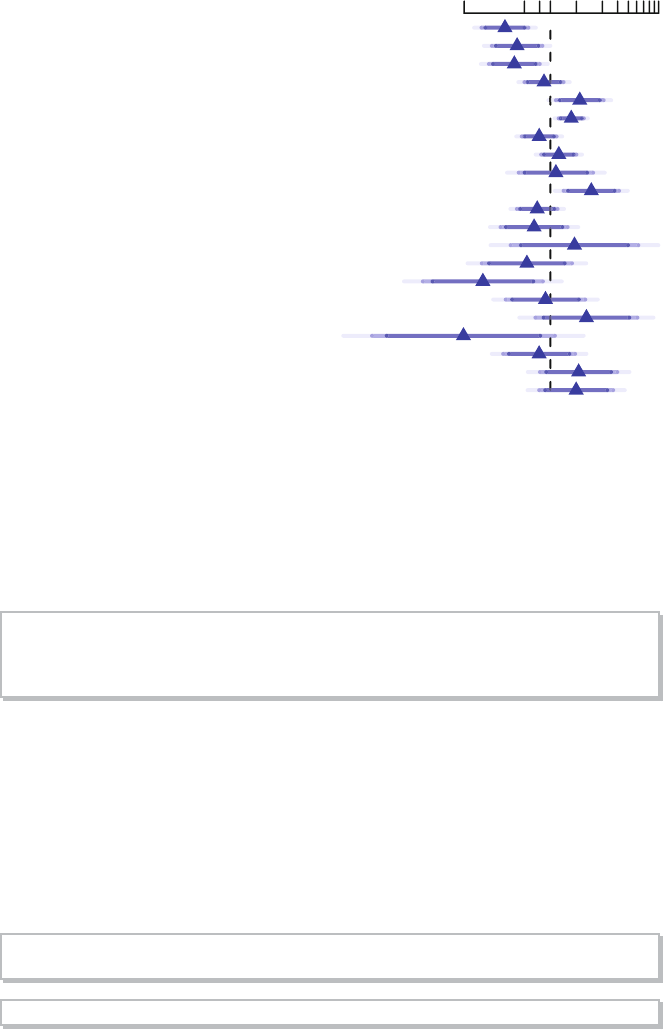
282 11 Binary Logistic Regression Case Study 1

Odds Ratio

0.10 0.50 2.00 8.00

sz − 25:6

sg − 12:9

ap − 7:0.5999756

sbp − 16:13

dbp − 9:7

age − 76:70

wt − 106:89

hg − 14.59961:12

bm − 1:0

hx − 1:0

dtime − 37:11

ekg − nrml:hrts

ekg − bngn:hrts

ekg − rd&ec:hrts

ekg − hbocd:hrts

ekg − MI:hrts

pf − in bed < 50% daytime:normal activity

pf − in bed > 50% daytime:normal activity

rx − 0.2 mg estrogen:placebo

rx − 1.0 mg estrogen:placebo

rx − 5.0 mg estrogen:placebo

Fig. 11.3 Interquartile-range odds ratios for continuous predictors and simple odds

ratios for categorical predictors. Numbers at left are upper quartile : lower quartile or

current group : reference group. The bars represent 0.9, 0.95, 0.99 conﬁdence limits.

The intervals are drawn on the log odds ratio scale and labeled on the odds ratio

scale. Ranges are on the original scale.

nom ← nomogram(fred , ap=c(.1, .5, 1, 5, 10, 50),

fun=plogis , funlabel="Probability ",

fun.at =c(.01 ,.05 ,.1,.25 ,.5,.75 ,.9,.95,.99))

plot(nom , xfrac=.45) # Figure 11.4

It is readily seen from this model that patients with a history of heart

disease, and patients with less extensive prostate cancer are those more likely

to die from cvd rather than from cancer. But beware that it is easy to over-

interpret ﬁndings when using unpenalized estimation, and conﬁdence inter-

vals a re too narrow. Let us use the bootstrap to study the uncertainty in

the selection of variables and to penalize fo r this uncertainty when estimat-

ing predictive performance of the model. The variables selected in the ﬁrst 20

bootstrap resamples are shown, making it obvious that the set of “signiﬁcant”

variables, i.e., the ﬁnal model, is somewhat a rbitrary.

f ← update (f, x=TRUE , y=TRUE)

v ← validate(f, B=200, bw=TRUE)

latex(v, B=20, digits =3)

11.6 Backwards Step-Down 283

Points

0 102030405060708090100

Size of Primary Tumor

(cm^2)

70 65 60 55 50 45 40 35 30 25 20 15 10 5 0

Serum Prostatic Acid

Phosphatase

50 10 5 1 0.5 0.1

ge in Years

45 50 55 60 65 70 75 80 85 90

History of Cardiovascular

Disease

Total Points

0 50 100 150 200 250 300

Linear Predictor

−5 −4 −3 −2 −1 0 1 2 3 4

Probability

0.01 0.05 0.1 0.25 0.5 0.75 0.9 0.95

Fig. 11.4 Nomogram calculating X

β and

P for cvd as the cause of death, using

the step-down model. For each predictor, read the points assigned on the 0–100 scale

and add these points. Read the result on the Total Points scale and then read the

corresponding predictions below it.

Index Original Training Test O ptimism Co rrected n

Sample Sample Sample Index

0.682 0.713 0.643 0.071 0.611 200

0.439 0.481 0.393 0.088 0.351 200

Intercept 0.000 0.000 −0.006 0.006 −0.006 200

Slope 1.000 1.000 0.811 0.189 0.811 200

max

0.000 0.000 0.048 0.048 0.048 200

D 0.395 0.449 0.346 0.102 0.293 200

U −0.008 −0.008 0.018 −0.026 0.018 200

Q 0.403 0.456 0.329 0.128 0.275 200

B 0.162 0.151 0.174 −0.022 0.184 200

g 1.932 2.213 1.756 0.457 1.475 200

0.341 0.355 0.320 0.035 0.306 200

284 11 Binary Logistic Regression Case Study 1

Fa ctors Retained in Backwards Elimination

First 20 Resamples

sz sg ap sbp dbp age wt hg ekg pf bm hx rx dtime

•••

•• ••• • ••

•• ••

••

•• • •

••

•• •••

•• ••

•• •

•• • •

•• ••

•• • • • • • •

••• •

••• • • •

••

•• • •

••

Frequencies of Numbers of Factors Retained

1234567891112

63947611910842 3 1

The slop e shrinkage (ˆγ) is a bit lower than was estimated above. There is

drop-oﬀ in all indexes. The estimated likely future predictive discrimination

of the model as measured by Somers’ D

fell from 0.682 to 0.611. The

latter estimate is the one that should be claimed when describing model

performance.

A nearly unbiased estimate of future calibratio n of the stepwise-derived

model is g iven below.

cal ← calibrate(f, B=200, bw=TRUE)

plot(cal) # Figure 11.5

The amount of overﬁtting seen in Figure 11.5 is consistent with the indexes

produced by the validate function.

For compari son, consider a bootstrap validation of the full model without

using variable selection.

vfull ← validate(f, B=200)

latex(vfull , digits =3)

11.6 Backwards Step-Down 285

0.0 0.2 0.4 0.6 0.8 1.0

0.0

0.2

0.4

0.6

0.8

1.0

Predicted Pr{cvd}

Actual Probability

Mean absolute error=0.028 n=257B= 200 repetitions, boot

Apparent

Bias−corrected

Ideal

Fig. 11.5 Bootstrap overﬁtting–corrected calibration curve estimate for the back-

wards step-down cause of death logistic model, along with a rug plot showing the dis-

tribution of predicted risks. The smooth nonparametric calibration estimator (loess)

is used.

Index Original Training Test O ptimism Co rrected n

Sample Sample Sample Index

0.786 0.833 0.738 0.095 0.691 200

0.573 0.641 0.501 0.140 0.433 200

Intercept 0.000 0.000 −0.013 0.013 −0.013 200

Slope 1.000 1.000 0.690 0.310 0.690 200

max

0.000 0.000 0.085 0.085 0.085 200

D 0.558 0.653 0.468 0.185 0.373 200

U −0.008 −0.008 0.051 −0.058 0.051 200

Q 0.566 0.661 0.417 0.244 0.322 200

B 0.133 0.115 0.150 −0.035 0.168 200

g 2.688 3.464 2.355 1.108 1.579 200

0.394 0.416 0.366 0.050 0.344 200

Compared to the validation of the full model, the step-down model has less

optimism, but it started with a smaller D

due to loss of information from

removing moderately important variables. The impr ovement in optimism was

not enough to oﬀset the eﬀect of eliminating variables. If shrinkage were used

with the full model, it would have better ca libration and discrimination than

the reduced model, since shrinkage does not diminish D

. Thus stepwise

variable selection failed at delivering excellent predictive discrimination.

Finally, compare previous results with a bootstrap validation of a step-

down model using a better signiﬁcance level for a variable to stay in the

286 11 Binary Logistic Regression Case Study 1

model (α =0.5,

589

) and using individual approximate Wald tests rather

than tests combining all deleted variables.

v5 ← validate(f, bw=TRUE , sls=0.5, type= ' individual ' , B=200)

Backwards Step-down - Original Model

Deleted Chi-Sq d.f. P Residual d.f. P AIC

ekg 6.76 5 0.2391 6.76 5 0.2391 -3.24

bm 0.09 1 0.7639 6.85 6 0.3349 -5.15

hg 0.38 1 0.5378 7.23 7 0.4053 -6.77

sbp 0.48 1 0.4881 7.71 8 0.4622 -8.29

wt 1.11 1 0.2932 8.82 9 0.4544 -9.18

dtime 1.47 1 0.2253 10.29 10 0.4158 -9.71

rx 5.65 3 0.1302 15.93 13 0.2528 -10.07

Approximate Estimates after Deleting Factors

Coef S.E. Wald Z P

Intercept -4.86308 2.67292 -1.819 0.068852

sz -0.05063 0.01581 -3.202 0.001366

sg -0.28038 0.11014 -2.546 0.010903

ap -0.24838 0.12369 -2.008 0.044629

dbp 0.28288 0.13036 2.170 0.030008

age 0.08502 0.02690 3.161 0.001572

pf=in bed < 50% daytime 0.81151 0.66376 1.223 0.221485

pf=in bed > 50% daytime -2.19885 1.21212 -1.814 0.069670

hx 0.87834 0.35203 2.495 0.012592

Factors in Final Model

[1] sz sg ap dbp age pf hx

latex(v5, digits =3, B=0)

Index Original Training Test O ptimism Co rrected n

Sample Sample Sample Index

0.739 0.801 0.716 0.085 0.654 200

0.517 0.598 0.481 0.117 0.400 200

Intercept 0.000 0.000 −0.008 0.008 −0.008 200

Slope 1.000 1.000 0.745 0.255 0.745 200

max

0.000 0.000 0.067 0.067 0.067 200

D 0.486 0.593 0.444 0.149 0.337 200

U −0.008 −0.008 0.033 −0.040 0.033 200

Q 0.494 0.601 0.411 0.190 0.304 200

B 0.147 0.125 0.156 −0.030 0.177 200

g 2.351 2.958 2.175 0.784 1.567 200

0.372 0.401 0.358 0.043 0.330 200

The performance statistics are midway between the full model and the

smaller stepwise model.

11.7 Model Approximation 287

11.7 Model Approximation

Frequently a better approach than stepwise variable selection is to approx-

imate the full model, using its estimates of precision, as discussed in Sec-

tion

5.5. Stepwise variable selection as well as regression trees are useful for

making the approximations, and the sacriﬁce in predictive accuracy is always

apparent.

We begin by computing the “gold standard” linear predictor from the full

model ﬁt (R

=1.0), then r unning backwards step-down OLS regression to

approximate it.

lp ← predict(f) # Compute linear predictor from full model

# Insert sigma=1 as otherwise sigma=0 will cause problems

a ← ols(lp ∼ sz + sg + log(ap) + sbp + dbp + age + wt +

hg + ekg + pf + bm + hx + rx + dtime , sigma =1,

data=psub)

# Specify silly stopping criterion to remove all variables

s ← fastbw (a, aics =10000)

betas ← s$Coefficients # matrix , rows=iterations

X ← cbind (1, f$x) # design matrix

# Compute the series of approximations to lp

ap ← X %*% t(betas )

# For each approx. compute approximation R

∧

2 and ratio of

# likelihood ratio chi-square for approximate model to that

# of original model

m ← ncol(ap) - 1 # all but intercept-only model

r2 ← frac ← numeric(m)

fullchisq ← f$stats[ ' Model L.R. ' ]

for(i in 1:m) {

lpa ← ap[,i]

r2[i] ← cor(lpa , lp)

∧

fapprox ← lrm(cvd ∼ lpa , data=psub)

frac[i] ← fapprox$stats [ ' Model L.R. ' ] / fullchisq

} # Figure 11.6:

plot(r2, frac , type= ' b ' ,

xlab=expression (paste( ' Approximation ' ,R

∧

2)),

ylab=expression (paste( ' Fraction of ' ,

chi

∧

2, ' Preserved ' )))

abline (h=.95 , col=gray(.83)); abline (v=.95 , col=gray(.83))

abline (a=0, b=1, col=gray(.83))

After 6 deletions, slightly more than 0.05 of both the LR χ

and the approx-

imation R

are lost (see Figure

11.6). Therefore we take as our approximate

model the one that removed 6 predictors. The equation for this model is

below, and its nomogram is in Figure

11.7.

fapprox ← ols(lp ∼ sz + sg + log(ap) + age + ekg + pf + hx +

rx, data=psub)

fapprox$stats [ ' R2 ' ] # as a check

R2 0.9453396

latex(fapprox , file= '')

288 11 Binary Logistic Regression Case Study 1

0.5 0.6 0.7 0.8 0.9 1.0

0.4

0.5

0.6

0.7

0.8

0.9

1.0

Approximation R

Fraction of χ

Preserved

Fig. 11.6 Fraction of explainable variation (full model LR χ

)incvd that was

explained by approximate models, along with approximation accuracy (x–axis)

E(lp) = Xβ, where

β =

−2.868303 − 0.06233241 sz − 0.3157901 sg − 0.3834479 log(ap) + 0.09089393 age

+1.396922[bngn] + 0.06275034[rd&ec] − 1.24892[hbocd] + 0.6511938[hrts]

+0.3236771[MI]

+1.116028[in bed < 50% daytime] − 2.436734[in bed > 50% daytime]

+1.05316 hx

−0.3888534[0.2 mg estrogen] + 0.6920495[1.0 mg estrogen]

+0.7834498[5.0 mg estrogen]

and [c] = 1 if subject is in group c, 0otherwise.

nom ← nomogram(fapprox , ap=c(.1, .5, 1, 5, 10, 20, 30, 40),

fun=plogis , funlabel="Probability ",

lp.at =(-5):4,

fun.lp.at=qlogis (c(.01 ,.05 ,.25 ,.5,.75 ,.95 ,.99)))

plot(nom , xfrac=.45) # Figure 11.7

11.7 Model Approximation 289

Points

0 102030405060708090100

Size of Primary Tumor

(cm^2)

70 65 60 55 50 45 40 35 30 25 20 15 10 5 0

Combined Index of Stage

and Hist. Grade

15 14 13 12 11 10 9 8 7 6 5

Serum Prostatic Acid

Phosphatase

40 10 5 1 0.5 0.1

ge in Years

45 50 55 60 65 70 75 80 85 90

ekg

hbocd rd&ec hrts

nrml bngn

in bed > 50% daytime in bed < 50% daytime

normal activity

History of Cardiovascular

Disease

0.2 mg estrogen

placebo

Total Points

0 50 100 150 200 250 300 350 400

Linear Predictor

−5 −3 −1 0 1 2 3 4

Probability

0.01 0.05 0.250.50.75 0.95 0.99

Fig. 11.7 Nomogram for predicting the probability of cvd based on the approximate

model

Chapter 12

Logistic Model Case Study 2: Survival

of Titanic Passengers

This case study demonstrates the development of a binary logistic regression

model to describe patterns of survival in passengers on the Titanic, based on

passenger age, sex, ticket class, and the number of family members accom-

panying each passenger. Nonparametric regression is also used. Since many

of the passengers had missing ages, multiple imputation is used so tha t the

complete information on the other variables can be e ﬃciently utilized. Titanic

passenger data were gathered by many researchers. Primary references are

the Encyclopedia Titanica at

www.encyclopedia-titanica.org and Eaton and

Haas.

169

Titanic survival patterns have been analyzed previously

151, 296, 571

but without incorporation of individual passenger ages. Thomas Cason while

a University of Virginia student co mpiled and interpreted the data from the

World Wide Web. One thousand three hundred nine of the passengers are

represented in the dataset, which is available from this text’s Web site under

the name titanic3. An early analysis of Titanic data may be found in Bron

12.1 Descriptive Statistics

First we obtain basic descriptive statistics o n key variables.

require(rms)

getHdata(titanic3) # get dataset from web site

# List of names of variables to analyze

v ← c( ' pclass ' , ' survived ' , ' age ' , ' sex ' , ' sibsp ' , ' parch ' )

t3 ← titanic3[, v]

units(t3$age) ← ' years '

latex(describe(t3), file= '')

F.E. Harrell, Jr., Regression Modeling Strategies, Springer Series

in Statistics, DOI 10.1007/978-3-319-19425-7

291

292 12 Logistic Model Case Study 2: Survival of Titanic Passengers

6 Variables 1309 Observations

pclass

n missing unique

1309 0 3

1st (323, 25%), 2nd (277, 21%), 3rd (709, 54%)

survived : Survived

n missing unique Info Sum Mean

1309 0 2 0.71 500 0.382

age : Age [years]

n missing unique Info Mean .05 .10 .25 .50 .75 .90 .95

1046 263 98 1 29.88 5 14 21 28 39 50 57

lowest : 0.1667 0.3333 0.4167 0.6667 0.7500

highest: 70.5000 71.0000 74.0000 76.0000 80.0000

sex

n missing unique

1309 0 2

female (466, 36%), male (843, 64%)

sibsp : Number of Siblings/Spouses Aboard

n missing unique Info Mean

1309 0 7 0.67 0.4989

0 123458

Frequency 891 319 42 20 22 6 9

% 682432201

parch : Number of Parents/Children Aboard

n missing unique Info Mean

1309 0 8 0.55 0.385

0 1 234569

Frequency 1002 170 113 86622

% 77 13 910000

Next, we obtain access to the needed variables and observations, and save data

distribution characteristics for plotting and for computing predictor eﬀects.

There are not many passengers having more than 3 siblings or spouses or

more than 3 children, so we truncate two variables at 3 for the purpose of

estimating stratiﬁed survival probabilities.

dd ← datadist(t3)

# describe distributions of variables to rms

options(datadist= ' dd ' )

s ← summary(survived ∼ age + sex + pclass +

cut2(sibsp ,0:3) + cut2(parch ,0:3), data=t3)

plot(s, main= '', subtitles=FALSE) # Figure 12.1

Note the large number of missing ages. Also note the strong eﬀects of sex and

passenger class on the probability of surviving. The age eﬀect do es not appear

to be very strong, because as we show later, much of the eﬀect is restricted to

12.1 Descriptive Statistics 293

Survived

0.2 0.3 0.4 0.5 0.6 0.7

1309

113

170

1002

319

891

709

277

323

843

466

263

245

265

246

290

Missing

female

male

1st

2nd

3rd

[ 0.167,22.0)

[22.000,28.5)

[28.500,40.0)

[40.000,80.0]

[3,8]

[3,9]

Age [years]

sex

pclass

Number of Siblings/Spouses Aboard

Number of Parents/Children Aboard

Overall

Fig. 12.1 Univariable summaries of Titanic survival

age < 21 years for one of the sexes. The eﬀects o f the last two variables are

unclear as the estimated proportions are not monotonic in the values of these

descriptors. Although some of the cell sizes are small, we can show four-way

empirical relationships with the fraction of surviving passengers by cr eating

four cells for sibsp × parch combinations and by creating two age groups. We

suppress proportions based on fewer than 25 passengers in a cell. Results are

shown in Figure

12.2.

tn ← transform(t3,

agec = ifelse (age < 21, ' child ' , ' adult ' ),

sibsp= ifelse (sibsp == 0, ' no sib/sp ' , ' sib/sp ' ),

parch= ifelse (parch == 0, ' no par/child ' , ' par/child ' ))

g ← function(y) if(length (y) < 25) NA else mean(y)

s ← with(tn, summarize(survived ,

llist(agec , sex , pclass , sibsp , parch ), g))

# llist , summarize in Hmisc package

# Figure 12.2:

ggplot (subset (s, agec != ' NA ' ),

aes(x=survived , y=pclass , shape=sex)) +

geom_point() + facet_grid(agec ∼ sibsp * parch ) +

xlab( ' Proportion Surviving ' ) + ylab( ' Passenger Class ' )+

scale_x_continuous (breaks =c(0, .5, 1))

294 12 Logistic Model Case Study 2: Survival of Titanic Passengers

1st

2nd

3rd

1st

2nd

3rd

adult

child

0.0 0.5

1.0

0.0

0.5 1.0 0.0 0.5 1.0 0.0 0.5 1.0

Proportion Surviving

Passenger Class

sex

female

male

no sib/sp

no par/child

no sib/sp

par/child

sib/sp

no par/child

sib/sp

par/child

Fig. 12.2 Multi-way summary of Titanic survival

Note that none of the eﬀects of sibsp or parch for common passenger groups

appear strong on an absolute risk scale.

12.2 Exploring Trends with Nonparametric Regression

As described in Section

2.4.7,theloess smoother has excellent performance

when the response is binary, as long as outlier detection is turned oﬀ. Here

we use a ggplot2 add-on function histSpikeg in the Hmisc package to obtain

and plot the loess ﬁt and age distribution. histSpikeg uses the “no iteration”

option for the R lowess function when the response is binary.

# Figure 12.3

b ← scale_size_discrete (range =c(.1, .85))

yl ← ylab(NULL)

p1 ← ggplot (t3, aes(x=age , y=survived)) +

histSpikeg(survived ∼ age , lowess =TRUE , data=t3) +

ylim(0,1) + yl

p2 ← ggplot (t3, aes(x=age , y=survived , color =sex)) +

histSpikeg(survived ∼ age + sex , lowess =TRUE ,

data=t3) + ylim(0,1) + yl

p3 ← ggplot (t3, aes(x=age , y=survived , size=pclass )) +

histSpikeg(survived ∼ age + pclass , lowess =TRUE ,

data=t3) + b + ylim (0,1) + yl

p4 ← ggplot (t3, aes(x=age , y=survived , color =sex ,

size=pclass )) +

histSpikeg(survived ∼ age + sex + pclass ,

lowess =TRUE , data=t3) +

b + ylim(0,1) + yl

gridExtra::grid.arrange (p1, p2, p3, p4, ncol =2) # combine 4

12.2 Exploring Trends with Nonparametric Regression 295

0.00

0.25

0.50

0.75

1.00

020406080

age

0.00

0.25

0.50

0.75

1.00

020406080

age

sex

female

male

0.00

0.25

0.50

0.75

1.00

020406080

age

pclass

1st

2nd

3rd

0.00

0.25

0.50

0.75

1.00

020406080

age

pclass

1st

2nd

3rd

sex

female

male

Fig. 12.3 Nonparametric regression (loess) estimates of the relationship between

age and the probability of s urviving the Titanic, with tick marks depicting the age

distribution. The top left panel shows unstratiﬁed estimates of the probability of

survival. Other panels show nonparametric estimates by various stratiﬁcations.

Figure

12.3 shows much of the story of passenger survival patterns. “Women

and children ﬁrst” seems to be true except for women in third class. It is

interesting tha t there is no real cutoﬀ for who is considered a child. For men,

the younger the greater chance of surviving. The interpretation of the eﬀects

of the “number of relatives”-type variables will be more diﬃcult, as their

deﬁnitions are a function of age. Figure 12.4 shows these relationships.

# Figure 12.4

top ← theme (legend.position = ' top ' )

p1 ← ggplot (t3, aes(x=age , y=survived , color =cut2(sibsp ,

0:2))) + stat_plsmo () + b + ylim(0,1) + yl + top +

scale_color_discrete (name= ' siblings/spouses ' )

296 12 Logistic Model Case Study 2: Survival of Titanic Passengers

p2 ← ggplot (t3, aes(x=age , y=survived , color =cut2(parch ,

0:2))) + stat_plsmo () + b + ylim(0,1) + yl + top +

scale_color_discrete (name= ' parents/children ' )

gridExtra::grid.arrange (p1, p2, ncol =2)

0.00

0.25

0.50

0.75

1.00

0 20406080

age

siblings/spouses 0 1 [2,8]

0.00

0.25

0.50

0.75

1.00

0 20406080

age

parents/children 0 1 [2,9]

Fig. 12.4 Relationship between age and survival stratiﬁed by the number of siblings

or spouses on board (left panel) or by the number of paren ts or children of the

passenger on board (right panel).

12.3 Binary Logistic Model With Casewise Deletion

of Missing Values

What follows is the standard analysis based on eliminating observations hav-

ing any missing data. We develop an initial somewhat saturated logistic

model, allowing for a ﬂexible nonlinear age eﬀect that can diﬀer in shape

for all six sex × class strata. The sibsp and parch variables do not have suf-

ﬁciently dispersed distributions to allow for us to model them nonlinearly.

Also, there are too few passengers with nonzero values of these two variables

in sex × pclass × age strata to allow us to model complex interactions in-

volving them. The meaning of these variables does depend on the passenger’s

age, so we consider only age interactions involving sibsp and parch.

f1 ← lrm(survived ∼ sex*pclass *rcs(age ,5) +

rcs(age ,5)*(sibsp + parch ), data=t3) # Table 12.1

latex(anova(f1), file= '', label = ' titanic-anova3 ' ,

size= ' small ' )

Three-way interactions are clearly insigniﬁcant (P =0.4) in Table 12.1.So

is parch (P =0.6 for testing the combined main eﬀect + interaction eﬀects

for parch, i.e., whether parch is important for any age). These eﬀects would

be deleted in almost all bootstrap resamples had we bo o tstrapp ed a variable

selection procedure using α =0.1forretentionofterms,sowecansafely

ignore these terms for future s teps. The model not containing those terms

12.3 Binary Logistic Model With Casewise Deletion of Missing Values 297

Table 12.1 Wald Statistics for survived

d.f. P

sex (Factor+Higher Order Factors) 187.15 15 < 0.0001

All Interactions 59.74 14 < 0.0001

pclass (Factor+Higher Order Factors) 100.10 20 < 0.0001

All Interactions 46.51 18 0.0003

age (Factor+Higher Order Factors) 56.20 32 0.0052

All Interactions 34.57 28 0.1826

Nonlinear (Factor+Higher Order Factors) 28.66 24 0.2331

sibsp (Factor+Higher Order Factors) 19.67 5 0.0014

All Interactions 12.13 4 0.0164

parch (Factor+Higher Order Factors) 3.51 5 0.6217

All Interactions 3.51 4 0.4761

sex × pclass (Factor+Higher Order Factors) 42.43 10 < 0.0001

sex × age (Factor+Higher Order Factors) 15.89 12 0.1962

Nonlinear (Factor+Higher Order Factors) 14.47 9 0.1066

Nonlinear Interaction : f(A,B) vs. AB 4.17 3 0.2441

pclass × age (Factor+Higher Order Factors) 13.47 16 0.6385

Nonlinear (Factor+Higher Order Factors) 12.92 12 0.3749

Nonlinear Interaction : f(A,B) vs. AB 6.88 6 0.3324

age × sibsp (Factor+Higher Order Factors) 12.13 4 0.0164

Nonlinear 1.76 3 0.6235

Nonlinear Interaction : f(A,B) vs. AB 1.76 3 0.6235

age ×

parch (Factor+Higher Order Factors) 3.51 4 0.4761

Nonlinear 1.80 3 0.6147

Nonlinear Interaction : f(A,B) vs. AB 1.80 3 0.6147

sex × pclass × age (Factor+Higher Order Factors) 8.34 8 0.4006

Nonlinear 7.74 6 0.2581

TOTAL NONLINEAR 28.66 24 0.2331

TOTAL INTERACTION 75.61 30 < 0.0001

TOTAL NONLINEAR + INTERACTION 79.49 33 < 0.0001

TOTAL 241.93 39 < 0.0001

is ﬁtted below. The ^2 in the model formula means to expand the terms in

parentheses to include all main eﬀects and second-order interactions.

f ← lrm(survived ∼ (sex + pclass + rcs(age ,5))

∧

rcs(age ,5)*sibsp , data=t3)

print(f, latex =TRUE)

Logistic Regression Model

lrm(formula = survived ~ (sex + pclass + rcs(age, 5))^2

+ rcs(age, 5) * sibsp, data = t3)

Frequencies of Missing Values Due to Each Variable

survived sex pclass age sibsp

0 0 0 263 0

298 12 Logistic Model Case Study 2: Survival of Titanic Passengers

Model Likelihood Discrimination Rank Discrim.

Ratio Test Indexes Indexes

Obs 1046 LR χ

553.87 R

0.555 C 0.878

0 619 d.f. 26 g 2.427 D

0.756

1 427 Pr(>χ

) < 0.0001 g

11.325 γ 0.758

max |

∂ log L

∂β

| 6×10

−6

0.365 τ

0.366

Brier 0.130

Coef S.E. Wald Z Pr(> |Z|)

Intercept 3.3075 1.8427 1.79 0.0727

sex=male -1.1478 1.0878 -1.06 0.2914

pclass=2nd 6.7309 3.9617 1.70 0.0893

pclass=3rd -1.6437 1.8299 -0.90 0.3691

age 0.0886 0.1346 0.66 0.5102

age’ -0.7410 0.6513 -1.14 0.2552

age” 4.9264 4.0047 1.23 0.2186

age”’ -6.6129 5.4100 -1.22 0.2216

sibsp -1.0446 0.3441 -3.04 0.0024

sex=male * pclass=2nd -0.7682 0.7083 -1.08 0.2781

sex=male * pclass=3rd 2.1520 0.6214 3.46 0.0005

sex=male * age -0.2191 0.0722 -3.04 0.0024

sex=male * age’ 1.0842 0.3886 2.79 0.0053

sex=male * age” -6.5578 2.6511 -2.47 0.0134

sex=male * age”’ 8.3716 3.8532 2.17 0.0298

pclass=2nd * age -0.5446 0.2653 -2.05 0.0401

pclass=3rd * age -0.1634 0.1308 -1.25 0.2118

pclass=2nd * age’ 1.9156 1.0189 1.88 0.0601

pclass=3rd * age’ 0.8205 0.6091 1.35 0.1780

pclass=2nd * age” -8.9545 5.5027 -1.63 0.1037

pclass=3rd * age” -5.4276 3.6475 -1.49 0.1367

pclass=2nd * age”’ 9.3926 6.9559 1.35 0.1769

pclass=3rd * age”’ 7.5403 4.8519 1.55 0.1202

age * sibsp 0.0357 0.0340 1.05 0.2933

age’ * sibsp -0.0467 0.2213 -0.21 0.8330

age” * sibsp 0.5574 1.6680 0.33 0.7382

age”’ * sibsp -1.1937 2.5711 -0.46 0.6425

latex(anova(f),file= '',label = ' titanic-anova2 ' ,size= ' small ' )

#12.2

This is a very powerful model (ROC area = c =0.88); the survival patterns

are easy to detect. The Wa ld ANOVA in Table 12.2 indicates especially strong

sex and pclass eﬀects (χ

= 199 and 109, respectively). There is a very strong

12.3 Binary Logistic Model With Casewise Deletion of Missing Values 299

Table 12.2 Wald Statistics for survived

d.f. P

sex (Factor+Higher Order Factors) 199.42 7 < 0.0001

All Interactions 56.14 6 < 0.0001

pclass (Factor+Higher Order Factors) 108.73 12 < 0.0001

All Interactions 42.83 10 < 0.0001

age (Factor+Higher Order Factors) 47.04 20 0.0006

All Interactions 24.51 16 0.0789

Nonlinear (Factor+Higher Order Factors) 22.72 15 0.0902

sibsp (Factor+Higher Order Factors) 19.95 5 0.0013

All Interactions 10.99 4 0.0267

sex × pclass (Factor+Higher Order Factors) 35.40 2 < 0.0001

sex × age (Factor+Higher Order Factors) 10.08 4 0.0391

Nonlinear 8.17 3 0.0426

Nonlinear Interaction : f(A,B) vs. AB 8.17 3 0.0426

pclass × age (Factor+Higher Order Factors) 6.86 8 0.5516

Nonlinear 6.11 6 0.4113

Nonlinear Interaction : f(A,B) vs. AB 6.11 6 0.4113

age × sibsp (Factor+Higher Order Factors) 10.99 4 0.0267

Nonlinear 1.81 3 0.6134

Nonlinear Interaction : f(A,B) vs. AB 1.81 3 0.6134

TOTAL NONLINEAR 22.72 15 0.0902

TOTAL INTERACTION 67.

58 18 < 0.0001

TOTAL NONLINEAR + INTERACTION 70.68 21 < 0.0001

TOTAL 253.18 26 < 0.0001

sex × pclass interaction and a strong age × sibsp interaction, considering

the strength of sibsp overa ll.

Let us examine the shapes of predictor eﬀects. With so many interactions

in the model we need to obtain predicted values at least for all combinations

of sex and pclass.Forsibsp we consider only two of its possible values.

p ← Predict(f, age , sex , pclass , sibsp =0, fun=plogis )

ggplot (p) # Fig. 12.5

Note the agreement between the lower right-hand panel of Figur e 12.3 with

Figure 12.5. This results from our use of similar ﬂexibility in the parametric

and nonparametric approaches (and similar eﬀective degrees of freedom). The

estimated eﬀect of sibsp as a function of age is shown in Figure

12.6.

ggplot (Predict(f, sibsp , age=c(10,15,20,50), conf.int=FALSE ))

## Figure 12.6

Note that children having many siblings apparently had lower survival. Mar-

ried adults had slightly higher survival than unmarried ones.

There will never be another Titanic, so we do not need to validate the

model for prospective use. But we use the bootstrap to validate the model

anyway, in an eﬀort to detect whether it is overﬁtting the data. We do not

pe nalize the calculations that fo llow for having examined the eﬀect of

parch or

300 12 Logistic Model Case Study 2: Survival of Titanic Passengers

1st 2nd 3rd

0.00

0.25

0.50

0.75

1.00

020406002040600 204060

Age, years

sex

female

male

Fig. 12.5 Eﬀects of predictors on probability of survival of Titanic passengers, esti-

mated for zero siblings or spouses

−6

−5

−4

−3

−2

−1

02468

Number of Siblings/Spouses Aboard

log odds

Age, years

Fig. 12.6 Eﬀect of number of siblings and spouses on the log odds of surviving, for

third class males

for testing three-way interactions, in the belief that these tests would replicate

well.

f ← update (f, x=TRUE , y=TRUE)

# x=TRUE , y=TRUE adds raw data to fit object so can bootstrap

set.seed(131) # so can replicate re-samples

latex(validate(f, B=200), digits =2, size= ' Ssize ' )

12.3 Binary Logistic Model With Casewise Deletion of Missing Values 301

Index Original Training Test O ptimism Co rrected n

Sample Sample Sample Index

0.76 0.77 0.74 0.03 0.72 200

0.55 0.58 0.53 0.05 0.50 200

Intercept 0.00 0.00 −0.08 0.08 −0.08 200

Slope 1.00 1.00 0.87 0.13 0.87 200

max

0.00 0.00 0.05 0.05 0.05 200

D 0.53 0.56 0.50 0.06 0.46 200

U 0.00 0.00 0.01 −0.01 0.01 200

Q 0.53 0.56 0.49 0.07 0.46 200

B 0 .13 0.13 0.13 −0.01 0.14 200

g 2.43 2.75 2.37 0.37 2.05 200

0.37 0.37 0.35 0.02 0.35 200

cal ← calibrate(f, B=200) # Figure 12.7

plot(cal , subtitles=FALSE)

n=1046 Mean absolute error=0.009 Mean squared error=0.00012

0.9 Quantile of absolute error=0.017

The output of validate indicates minor overﬁtting. Overﬁtting would have

been worse had the risk factors not been so strong. The closeness of the cali-

bration curve to the 45

◦

line in Figure

12.7 demonstrates excellent validation

on a n absolute pro bability scale. But the extent of missing data casts some

doubt on the validity of this model, and on the eﬃciency of its parameter

estimates.

0.0 0.2 0.4 0.6 0.8 1.0

0.0

0.2

0.4

0.6

0.8

1.0

Predicted Pr{survived=1}

Actual Probability

Apparent

Bias−corrected

Ideal

Fig. 12.7 Bootstrap overﬁtting-corrected loess nonparametric calibration curve for

casewise deletion mo del

302 12 Logistic Model Case Study 2: Survival of Titanic Passengers

12.4 Examining Missing Data Patterns

The ﬁrst step to dealing with missing da ta is understanding the patterns

of missing values. To do this we use the Hmisc library’s naclus and naplot

functions, and the recursive partitioning library of Atkinson and Therneau.

Below naclus tells us which variables tend to be missing on the same persons,

and it computes the proportion of missing values for each variable. The rpart

function derives a tree to predict which types of passengers tended to have

age missing.

na.patterns ← naclus (titanic3)

require(rpart ) # Recursive partitioning package

who.na ← rpart (is.na(age) ∼ sex + pclass + survived +

sibsp + parch , data=titanic3 , minbucket =15)

naplot (na.patterns , ' na per var ' )

plot(who.na , margin =.1); text(who.na ) # Figure 12.8

plot(na.patterns )

We see in Figure 12.8 that age tends to be missing on the same passengers

as the body bag identiﬁer, and that it is missing in only 0.09 of ﬁrst or sec-

ond class passengers. The category of passengers having the highest fraction

of missing ages is third class passengers having no parents or children on

board. Below we use Hmisc’s summary.formula function to plot simple descrip-

tive statistics on the fraction of missing ages, stratiﬁed by other variables. We

see that without adjusting for other variables, age is slightly mor e missing on

nonsurviving passengers.

plot(summary(is.na(age) ∼ sex + pclass + survived +

sibsp + parch , data=t3)) # Figure 12.9

Let us derive a lo gistic model to predict missingness of age, to see if the

survival bias maintains after adjustment for the other variables.

m ← lrm(is.na(age) ∼ sex * pclass + survived + sibsp + parch ,

data=t3)

print(m, latex=TRUE, needspace = ' 2in ' )

Logistic Regression Model

lrm(formula = is.na(age) ~ sex * pclass + survived + sibsp +

parch, data = t3)

Model Likelihood Discrimination Rank Discrim.

Ratio Test Indexes Indexes

Obs 1309 LR χ

114.99 R

0.133 C 0.703

FALSE 1046 d.f. 8 g 1.015 D

0.406

TRUE 263 Pr(>χ

) < 0.0001 g

2.759 γ 0.452

max |

∂ log L

∂β

| 5×10

−6

0.126 τ

0.131

Brier 0.148

12.4 Examining Missing Data Patterns 303

Fraction of NAs in each Variable

Fraction of NAs

0.0 0.2 0.4 0.6 0.8

pclass

survived

name

sex

sibsp

parch

ticket

cabin

boat

fare

embarked

age

home.dest

body

pclass=ab

parch>=0.5

0.09167

0.1806 0.3249

boat

embarked

cabin

fare

ticket

parch

sibsp

age

body

home.dest

sex

name

pclass

survived

0.4

0.3

0.2

0.1

0.0

Fraction Missing

Fig. 12.8 Patterns of missing data. Upper left panel shows the fraction of observa-

tions missing on each predictor. Lower panel depicts a hierarchical cluster analysis of

missingness combinations. The similarity measure shown on the Y -axisisthefrac-

tion of observations for which both variables are missing. Right panel shows the result

of recursive partitioning for predicting is.na(age).Therpart function found only

strong patterns according to passenger class.

Coef S.E. Wald Z Pr(> |Z|)

Intercept -2.2030 0.3641 -6.05 < 0.0001

sex=male 0.6440 0.3953 1.63 0.1033

pclass=2nd -1.0079 0.6658 -1.51 0.1300

pclass=3rd 1.6124 0.3596 4.48 < 0.0001

survived -0.1806 0.1828 -0.99 0.3232

sibsp 0.0435 0.0737 0.59 0.5548

parch -0.3526 0.1253 -2.81 0.0049

sex=male * pclass=2nd 0.1347 0.7545 0.18 0.8583

sex=male * pclass=3rd -0.8563 0.4214 -2.03 0.0422

latex(anova(m), file= '', label= ' titanic-anova.na ' )

# Table 12.3

304 12 Logistic Model Case Study 2: Survival of Titanic Passengers

is.na(age)

0.0 0.2 0.4 0.6 0.8 1.0

1309

113

170

1002

319

891

500

809

709

277

323

843

466

female

male

1st

2nd

3rd

Yes

sex

pclass

Survived

Number of Siblings/Spouses Aboard

Number of Parents/Children Aboard

Overall

mean

Fig. 12.9 Univariable descriptions of proportion of passengers with missing age

Fortunately, after controlling for other variables, Table

12.3 provides evi-

dence that no nsurviving passengers ar e no more likely to have age missing.

The only important predictors of missingness are pclass and parch (the more

parents or children the passenger has on board, the less likely age was to be

missing).

12.5 Multiple Imputation

Multiple imputation is expected to r educe bias in estimates as well as to

provide an estimate of the va riance–covariance matrix of

β penalized for im-

putation. With multiple imputation, survival status can be used to impute

missing ages, so the age relationship will not be as attenuated as with single

conditional mean imputation.

aregImpute The following uses the Hmisc pack-

age aregImpute function to do predictive mean matching, using van Buuren’s

“Type 1” matching [

85, Section 3.4.2] in conjunction with bootstrapping to

incorporate all uncertainties, in the context of smooth additive imputation

12.5 Multiple Imputation 305

Table 12.3 Wald Statistics for is.na(age)

d.f. P

sex (Factor+Higher Order Fa ctors) 5.61 3 0.1324

All Interactions 5.58 2 0.0614

pclass (Factor+Higher Order Factors) 68.43 4 < 0.0001

All Interactions 5.58 2 0.0614

survived 0.98 1 0.3232

sibsp 0.35 1 0.5548

parch 7.92 1 0.0049

sex × pclass (Factor+Higher Order Factors) 5.58 2 0.0614

TOTAL 82.90 8 < 0.0001

models. Sampling of donors is handled by distance weighting to yield better

distributions of imputed values. By default, aregImpute does not transform

age when it is being predicted from the other variables. Four knots are used

to transform age when used to impute other variables (not needed here as no

other missings were present in the varia bles of interest). Since the fraction of

observations with missing age is

263

1309

=0.2 we use 20 imputations.

set.seed(17) # so can reproduce random aspects

mi ← aregImpute(∼ age + sex + pclass +

sibsp + parch + survived ,

data=t3, n.impute=20, nk=4, pr=FALSE)

Multiple Imputation using Bootstrap and PMM

aregImpute(formula = ∼age + sex + pclass + sibsp + parch + survived ,

data = t3, n.impute = 20, nk = 4, pr = FALSE)

n: 1309 p: 6 Imputations: 20 nk: 4

Number of NAs:

age sex pclass sibsp parch survived

26300000

type d.f.

age s 1

sex c 1

pclass c 2

sibsp s 2

parch s 2

survived l 1

Transformation of Target Variables Forced to be Linear

R-squares for Predicting Non-Missing Values for Each Variable

Using Last Imputations of Predictors

age

0.295

306 12 Logistic Model Case Study 2: Survival of Titanic Passengers

# Print the first 10 imputations for the first 10 passengers

# having missing age

mi$imputed$age[1:10, 1:10]

[,1] [,2] [,3] [,4] [,5] [,6] [,7] [,8] [,9] [,10]

16 40 49 24 29 60.0 58 64 36 50 61

38 33 45 40 49 80.0 2 38 38 36 53

41 29 24 19 31 40.0 60 64 42 30 65

47 40 42 29 48 36.0 46 64 30 38 42

60 52 40 22 31 38.0 22 19 24 40 33

70 16 14 23 23 18.0 24 19 27 59 23

71 30 62 57 30 42.0 31 64 40 40 63

75 43 23 36 61 45.5 58 64 27 24 50

81 44 57 47 31 45.0 30 64 62 39 67

107 52 18 24 62 32.5 38 64 47 19 23

plot(mi)

Ecdf(t3$age , add=TRUE , col= ' gray ' , lwd=2,

subtitles=FALSE)#Fig. 12.10

0 20406080

0.0

0.2

0.4

0.6

0.8

1.0

Imputed age

Proportion <= x

Fig. 12.10 Distributions of imputed and actual ages for the Titanic dataset. Imputed

values are in black and actual ages in gray.

We now ﬁt logistic models for ﬁve completed datasets. The fit.mult.impute

function ﬁts ﬁve models and examines the within– and between–imputation

variances to compute an imputation-corrected va riance–covariance matrix

that is stored in the ﬁt object f.mi. fit.mult.impute will also average the ﬁve

β vectors, storing the result in f.mi$coefficients. The function also prints

the ratio of imputation-corrected variances to average ordinary variances.

f.mi ← fit.mult.impute (

survived ∼ (sex + pclass + rcs(age ,5))

∧

rcs(age ,5)*sibsp ,

12.6 Summarizing the Fitted Model 307

Table 12.4 Wald Statistics for survived

d.f. P

sex (Factor+Higher Order Factors) 240.42 7 < 0.0001

All Interactions 54.56 6 < 0.0001

pclass (Factor+Higher Order Factors) 114.21 12 < 0.0001

All Interactions 36.43 10 0.0001

age (Factor+Higher Order Factors) 50.37 20 0.0002

All Interactions 25.88 16 0.0557

Nonlinear (Factor+Higher Order Factors) 24.21 15 0.0616

sibsp (Factor+Higher Order Factors) 24.22 5 0.0002

All Interactions 12.86 4 0.0120

sex × pclass (Factor+Higher Order Factors) 30.99 2 < 0.0001

sex × age (Factor+Higher Order Factors) 11.38 4 0.0226

Nonlinear 8.15 3 0.0430

Nonlinear Interaction : f(A,B) vs. AB 8.15 3 0.0430

pclass × age (Factor+Higher Order Factors) 5.30 8 0.7246

Nonlinear 4.63 6 0.5918

Nonlinear Interaction : f(A,B) vs. AB 4.63 6 0.5918

age × sibsp (Factor+Higher Order Factors) 12.86 4 0.0120

Nonlinear 1.84 3 0.6058

Nonlinear Interaction : f(A,B) vs. AB 1.84 3 0.6058

TOTAL NONLINEAR 24.21 15 0.0616

TOTAL INTERACTION 67.12 18 < 0.

0001

TOTAL NONLINEAR + INTERACTION 70.99 21 < 0.0001

TOTAL 298.78 26 < 0.0001

lrm , mi, data=t3, pr=FALSE )

latex(anova(f.mi), file= '', label= ' titanic-anova.mi ' ,

size= ' small ' ) # Table 12.4

The Wald χ

for age is reduced by accounting for imputation but is in-

creased (by a lesser amount) by using patterns of association with survival

status to impute missing age. The Wald tests are all adjusted for multiple im-

putation. Now examine the ﬁtted age relationship using multiple imputation

vs. casewise deletion.

p1 ← Predict(f, age , pclass , sex , sibsp =0, fun=plogis )

p2 ← Predict(f.mi , age , pclass , sex , sibsp =0, fun=plogis )

p ← rbind ( ' Casewise Deletion ' =p1, ' Multiple Imputation ' =p2)

ggplot (p, groups = ' sex ' , ylab= ' Probability of Surviving ' )

# Figure 12.11

12.6 Summarizing the Fitted Model

In this section we depict the model ﬁtted using multiple imputation, by com-

puting odds ratios and by showing various predicted values. For age, the odds

ratio for an increase from 1 year old to 30 years old is computed, instead of

the default odds ratio based on outer quartiles of age. The estimated odds

308 12 Logistic Model Case Study 2: Survival of Titanic Passengers

Casewise Deletion Multiple Imputation

0.00

0.25

0.50

0.75

1.00

0.00

0.25

0.50

0.75

1.00

0.00

0.25

0.50

0.75

1.00

1st

2nd

3rd

02040600204060

Age, years

Probability of Surviving

sex

female

male

Fig. 12.11 Predicted probability of s urvival for males from ﬁt using casewise deletion

again (top) and multiple random draw imputation (bottom). Both sets of predictions

are for sibsp=0.

ratios are very dependent on the levels of interacting factors, so Figure

12.12

depicts only one of many patterns.

# Get predicted values for certain types of passengers

s ← summary(f.mi , age=c(1,30), sibsp =0:1)

# override default ranges for 3 variables

plot(s, log=TRUE , main= '') # Figure 12.12

Now compute estimated probabilities of survival for a variety of settings of

the predictors.

12.6 Summarizing the Fitted Model 309

0.10 0.50 2.00 5.00

age − 30:1

sibsp − 1:0

sex − female:male

pclass − 1st:3rd

pclass − 2nd:3rd

Adjusted to:sex=male pclass=3rd age=28 sibsp=0

Fig. 12.12 Odds ratios for some predictor settings

phat ← predict(f.mi ,

combos ←

expand.grid(age=c(2,21,50), sex=levels (t3$sex),

pclass =levels (t3$pclass ),

sibsp =0), type= ' fitted ' )

# Can also use Predict(f.mi , age=c(2,21,50), sex, pclass ,

# sibsp=0, fun=plogis)$ yhat

options(digits =1)

data.frame(combos , phat)

age sex pclass sibsp phat

1 2 female 1st 0 0.97

2 21 female 1st 0 0.98

3 50 female 1st 0 0.97

4 2 male 1st 0 0.88

5 21 male 1st 0 0.48

6 50 male 1st 0 0.27

7 2 female 2nd 0 1.00

8 21 female 2nd 0 0.90

9 50 female 2nd 0 0.82

10 2 male 2nd 0 1.00

11 21 male 2nd 0 0.08

12 50 male 2nd 0 0.04

13 2 female 3rd 0 0.85

14 21 female 3rd 0 0.57

15 50 female 3rd 0 0.37

16 2 male 3rd 0 0.91

17 21 male 3rd 0 0.13

18 50 male 3rd 0 0.06

options(digits =5)

We can also get predicted values by creating an R function that will evaluate

the model on demand.

310 12 Logistic Model Case Study 2: Survival of Titanic Passengers

pred.logit ← Function(f.mi)

# Note: if don ' t define sibsp to pred.logit , defaults to 0

# normally just type the function name to see its body

latex(pred.logit , file= '', type= ' Sinput ' , size= ' small ' ,

width.cutoff =49)

pred.logit ← function (sex=”male”, pclass=”3rd”,

age = 28 , s ibsp = 0)

{

3.2427671 − 0.95431809 ∗ ( sex == ”male”) + 5.4086505 ∗

(pclass == ”2nd”) − 1.3378623 ∗ (pclass ==

”3rd ”) + 0 .091162649 ∗ age − 0 .00031204327 ∗

pmax( age − 6, 0)

∧

3 + 0 .0021750413 ∗ pmax( age −

21 , 0)

∧

3 − 0.0027627032 ∗ pmax( age − 27 , 0)

∧

0.0009805137 ∗ pmax( age − 36 , 0)

∧

3 − 8.0808484e−05 ∗

pmax( age − 55 . 8 , 0 )

∧

3 − 1.1567976 ∗ sibsp +

( s ex == ”male ”) ∗ ( −0.46061284 ∗ (pclass ==

”2nd”) + 2.0406523 ∗ (pclass == ”3rd”)) +

( s ex == ”male ”) ∗ ( −0.22469066 ∗ age + 0.00043708296 ∗

pmax( age − 6, 0)

∧

3 − 0.0026505136 ∗ pmax( age −

21 , 0)

∧

3 + 0.0031201404 ∗ pmax( age − 27 ,

∧

3 − 0.00097923749 ∗ pmax( age − 36 ,

∧

3 + 7 .2527708e−05 ∗ pmax( age − 55 . 8 ,

∧

3) + ( pclass == ”2nd”) ∗ ( −0.46144083 ∗

age + 0 .00070194849 ∗ pmax( age − 6, 0)

∧

3 −

0.0034726662 ∗ pmax( age − 21 , 0)

∧

3 + 0.0035255387 ∗

pmax( age − 27 , 0)

∧

3 − 0.0007900891 ∗ pmax( age −

36 , 0)

∧

3 + 3 .5268151e−05 ∗ pmax( age − 55 . 8 ,

∧

3) + ( pclass == ”3rd ”) ∗ ( −0.17513289 ∗

age + 0 .00035283358 ∗ pmax( age − 6, 0)

∧

3 −

0.0023049372 ∗ pmax( age − 21 , 0)

∧

3 + 0.0028978962 ∗

pmax( age − 27 , 0)

∧

3 − 0.00105145 ∗ pmax( age −

36 , 0)

∧

3 + 0.00010565735 ∗ pmax( age − 55 . 8 ,

∧

3) + sibsp ∗ (0 .040830773 ∗ age − 1 .5627772e−05 ∗

pmax( age − 6, 0)

∧

3 + 0 .00012790256 ∗ pmax( age −

21 , 0)

∧

3 − 0.00025039385 ∗ pmax( age − 27 ,

∧

3 + 0.00017871701 ∗ pmax( age − 36 , 0)

∧

3 −

4.0597949e−05 ∗ pmax( age − 55 .8 , 0 )

∧

}

# Run the newly created function

plogis (pred.logit(age=c(2,21,50), sex= ' male ' , pclass = ' 3rd ' ))

[1] 0.914817 0.132640 0.056248

A nomogram could be used to obtain predicted values manually, but this is

not feasible when so many interaction terms ar e present.

Chapter 13

Ordinal Logistic Regression

13.1 Background

Many medical and epidemiologic studies incorporate an ordinal response

variable. In some cases an ordinal response Y represents levels of a standard

measurement scale such as severity of pain (none, mild, moderate, severe).

In other cases, ordinal responses are constructed by specifying a hierarchy

of separate endpoints. For example, clinicians may sp ecify an ordering of

the severity of several component events and assign patients to the worst

event present from among none, heart attack, disabling stroke, and death.

Still another use of ordinal response methods is the application of rank-based

methods to continuous responses so as to obtain robust inferences. For ex-

ample, the proportional odds model described later a llows for a continuous

Y and is really a g eneralization of the Wilcoxon–Mann–Whitney rank test.

Thus the semiparametric pr oportional odds model is a direct competitor of

ordinary linear models.

There are many varia tions of logistic models used for predicting an ordinal

response variable Y . All of them have the advantage that they do not assume

a spacing between levels of Y . In other words, the same regression coeﬃcients

and P -values result fr om an analysis of a response var iable having levels 0, 1, 2

when the levels are recoded 0, 1, 20. Thus ordinal models use only the rank-

ordering of values of Y .

In this chapter we consider two of the most p o pular ordinal logistic models,

the proportional odds (PO) form of an ordinal logistic model

647

and the for-

ward continuation ratio (CR) ordinal logistic model.

190

Chapter 15 deals with

a wider variety of ordinal models with emphasis on analysis of continuous Y . 1

F.E. Harrell, Jr., Regression Modeling Strategies, Springer Series

in Statistics, DOI 10.1007/978-3-319-19425-7

311

312 13 Ordinal Logistic Regression

13.2 Ordinality Assumption

A basic assumption of all commonly used ordinal regression models is that the

response var iable behaves in a n ordinal fashion with respect to each predictor.

Assuming that a predictor X is linearly related to the log odds of some

appropriate event, a simple way to check for ordinality is to plot the mean

of X stratiﬁed by levels of Y . These means should be in a consistent order.

If for many of the Xs, two adjacent categories of Y do not distinguish the

means, that is evidence that those levels of Y should be pooled.

One can also estimate the mean or expected value of X|Y = j (E(X|Y =

j)) given that the ordinal model assumptions hold. This is a useful tool for

checking those assumptions, at least in an unadjusted fashion. For simplicity,

assume that X is discrete, and let P

=Pr(Y = j|X = x) be the probability

that Y = j given X = x that is dictated from the model being ﬁtted, with

X b eing the only predictor in the model. Then

Pr(X = x|Y = j)=Pr(Y = j|X = x)Pr(X = x)/Pr(Y = j)

E(X|Y = j)=



Pr(X = x)/ Pr(Y = j), (13.1)

and the expectation can be estimated by

E(X|Y = j)=



, (13.2)

where

denotes the estimate of P

from the ﬁtted one-predictor model

(for inner values of Y in the PO models, these probabilities are diﬀerences

between terms given by Equation

13.4 below), f

is the frequency of X = x

in the sample of size n,andg

is the frequency of Y = j in the sample. This

estimate can be computed conveniently without grouping the data by X.For

n subjects let the n values of X be x

,...,x

.Then

E(X|Y = j)=



i=1

. (13.3)

Note that if one were to compute diﬀerences between conditional means of X

and the conditional means of X given PO, and if furthermore the means were

conditioned on Y ≥ j instead of Y = j, the result would be proportional to

means of score residuals deﬁned later in Equation

13.6.

13.3 Prop ortional Odds Model 313

13.3 Proportional Odds Model

13.3.1 Model

The most commonly used ordinal logistic mo del was described in Walker

and Duncan

647

and later called the pr oportional odds (PO) model by Mc-

Cullagh.

449

The PO model is best stated as follows, for a response variable

having levels 0, 1, 2,...,k:

Pr[Y ≥ j|X]=

1+exp[−(α

+ Xβ)]

, (13.4)

where j =1, 2,...,k. Some authors write the model in terms of Y ≤ j.Our

formulation makes the model coeﬃcients consistent with the binary logistic

model. There are k intercepts (αs). For ﬁxed j, the model is an ordinary

logistic model for the event Y ≥ j. By using a common vector of regression

coeﬃcients β connecting probabilities for varying j, the PO model allows for

parsimonious modeling of the distribution of Y .

There is a nice connection between the PO model and the Wilcoxon–

Mann–Whitney two-sample test: when there is a single predictor X

that is

binary, the numerator of the score test for testing H

: β

= 0 is proportional

to the two-sample test statistic [

664, pp. 2258–2259].

13.3.2 Assumptions and Interpretation of Parameters

There is an implicit assumption in the PO model that the r egression coef-

ﬁcients (β) are independent of j, the cutoﬀ level for Y . One could say that

there is no X ×Y interaction if PO holds. For a speciﬁc Y -cutoﬀ j, the model

has the same assumptions as the binary logistic model (Section

10.1.1). That

is, the model in its simplest form assumes the log odds that Y ≥ j is linearly

related to each X and that there is no interaction between the Xs.

In designing clinical studies, one sometimes hear s the statement that an

ordinal outcome should be avoided since statistical tests of patterns of those

outcomes are hard to interpret. In fact, one interprets eﬀects in the PO model

using ordinary odds ratios. The diﬀerence is that a sing le odds ratio is as-

sumed to apply equally to all events Y ≥ j, j =1, 2,...,k. If linearity and

additivity hold, the X

+1:X

odds ratio for Y ≥ j is exp(β

), whatever

the cutoﬀ j.

The proportional hazards assumption is frequently violated, just as the as-

sumptions of normality o f residuals with equal variance in ordinary regression

are frequently violated, but the PO model can still be useful and powerful in

this situation. As stated by Senn and Julious

564

314 13 Ordinal Logistic Regression

Clearly, the dependence of the proportional odds model on the assumption

of proportionality can be over-stressed. Suppose that two diﬀerent statisticians

would cut the same three-point scale at diﬀerent cut points. It is hard to see how

anybody who could accept either dichotomy could object to the compromise

answer produced by the prop ortional odds model.

Sometimes it helps in interpreting the model to estimate the mean Y as

a function of one or more predictors, even though this assumes a spacing for

the Y -levels.3

13.3.3 Estimation

The PO model is ﬁtted using MLE on a somewhat complex likelihood function

that is dependent on diﬀerences in logistic model probabilities. The estimation

pro cess forces the αs to be in descending order.

13.3.4 Residuals

Schoenfeld residuals

557

are very eﬀective

233

in checking the proportional haz-

ards assumption in the Cox

132

survival model. For the PO model one could

analogously compute each subject’s contribution to the ﬁrst derivative of

the log likelihood function with respect to β

, average them separately by

levels of Y , and examine trends in the residual plots as in Section

20.6.2.

A few examples have shown that such plots are usually hard to interpret.

Easily interpreted score residual plots for the PO model can be constructed,

however, by using the ﬁtted PO model to predict a series of binary events

Y ≥ j, j =1, 2,...,k, using the corresponding predicted probabilities

1+exp[−(ˆα

+ X

β)]

, (13.5)

where X

stands for a vector of predictors for subject i. Then, after forming

an indicator variable for the event currently being predicted ([Y

≥ j]), one

computes the score (ﬁrst derivative) components U

from an ordinary binary

logistic model:

= X

([Y

≥ j] −

), (13.6)

for the subject i and predictor m. Then, for each column of U,plotthemean

·m

and conﬁdence limits, with Y (i.e., j)onthex-axis. For each predictor

the trend against j should be ﬂat if PO holds.

In binary logistic regression,

partial residuals are very useful as they allow the analyst to ﬁt linear eﬀects

β were derived from separate binary ﬁts, all

·m

≡ 0.

13.3 Prop ortional Odds Model 315

for all the predictors but then to nonparametrically estimate the true trans-

formation that each predictor requires (Section

10.4). The partial residual is

deﬁned as follows, for the ith subject and mth predictor variable.

115, 373

−

(1 −

)

, (13.7)

where

1+exp[−(α + X

β)]

. (13.8)

A smoothed plot (e.g., using the moving linear regression algorithm in

loess

111

)ofX

against r

provides a nonparametric estimate of how X

relates to the log relative odds that Y =1|X

. For ordinal Y , we just need

to compute binary model partial residuals for all cutoﬀs j:

≥ j] −

(1 −

)

, (13.9)

then to make a plot for each m showing smoothed partial residual curves for

all j, looking for similar shapes and slopes for a given predictor for all j.Each

curve provides an estimate of how X

relates to the relative log odds that

Y ≥ j. Since partial residuals allow examination of predictor transformations

(linearity) while simultaneously allowing examination of PO (parallelism),

partial residual plots are generally preferred over score residual plots for or-

dinal models.

Li and Shepherd

402

have a residual for ordinal models that serves for the

entire range of Y without the need to consider cutoﬀs. Their residual is use-

ful for checking functional form of predictors but not the proportional odds

assumption.

13.3.5 Assessment of Model Fit

Peterson and Harrell

502

developed score and likelihood ratio tests for testing

the PO a ssumption. The score test is used in the SAS PROC LOGISTIC,

540

but its extreme anti-conservatism in many cases can make it unreliable.

502

For determining whether the PO assumption is likely to be satisﬁed fo r

each predictor separately, there are several graphics that are useful. One is the

graph comparing means of X|Y with and without assuming PO, as described

in Section

13.2 (see Figure 14.2 for an example). Another is the simple method

of stratifying on each predictor and computing the logits of all proportions of

the form Y ≥ j, j =1, 2,...,k. When proportional odds holds, the diﬀerences

in logits between diﬀerent values of j should be the same at all levels of X,

316 13 Ordinal Logistic Regression

because the model dictates that logit(Y ≥ j|X) − logit(Y ≥ i|X)=α

− α

for any constant X. An example of this is in Figure

13.1.

require(Hmisc )

getHdata(support)

sfdm ← as.integer (support$sfdm2 ) - 1

sf ← function(y)

c( ' Y ≥ 1 ' =qlogis (mean(y ≥ 1)), ' Y ≥ 2 ' =qlogis (mean(y ≥ 2)),

' Y ≥ 3 ' =qlogis (mean(y ≥ 3)))

s ← summary(sfdm ∼ adlsc + sex + age + meanbp , fun=sf,

data=support)

plot(s, which =1:3, pch=1:3, xlab= ' logit ' , vnames = ' names ' ,

main= '', width.factor =1.5) # Figure 13.1

logit

−0.5 0.0 0.5 1.0 1.5

841

210

204

216

211

210

211

464

377

210

199

150

282

0.000

female

male

[0.495,1.167)

[1.167,3.024)

[3.024,7.000]

[19.8, 52.4)

[52.4, 65.3)

[65.3, 74.8)

[74.8,100.1]

[ 0, 64)

[ 64, 78)

[ 78,108)

[108,180]

adlsc

sex

age

meanbp

Overall

Fig. 13.1 Checking PO assumption separately for a series of predictors. The circle,

triangle, and plus sign correspond to Y ≥ 1, 2, 3, respectiv ely. PO is checked by

examining the vertical constancy of distances between any two of these three symbols.

Response variable is the severe functional disability scale sfdm2 from the 1000-patient

SUPPORT dataset, with the last two categories combined b ecause of low frequency

of coma/intubation.

When Y is co ntinuous or almost continuous and X is discrete, the PO model

assumes that the logit of the cumulative distribution function of Y is parallel

13.3 Prop ortional Odds Model 317

across categories of X. The corresponding, more rigid, assumptions of the

ordinar y linear mo del (here, parametric ANOVA) are parallelism and linear-

ity if the no rmal inver se cumulative distribution function across categories

of X. As an example consider the web site’s diabetes dataset, where we con-

sider the distribution of log glycohemoglobin across subjects’ body frames.

getHdata(diabetes)

a ← Ecdf(∼ log(glyhb), group =frame , fun=qnorm ,

xlab= ' log(HbA1c) ' , label.curves =FALSE , data=diabetes ,

ylab=expression (paste(Phi

∧

-1, (F[n](x))))) # Fig. 13.2

b ← Ecdf(∼ log(glyhb), group =frame , fun=qlogis ,

xlab= ' log(HbA1c) ' , label.curves =list(keys= ' lines ' ),

data=diabetes , ylab=expression(logit (F[n](x))))

print(a, more=TRUE , split =c(1,1,2,1))

print(b, split =c(2,1,2,1))

log(HbA1c)

−

(

x))

−2

1.0 1.5 2.0 2.5

log(HbA1c)

logit(F

(x))

−5

1.0 1.5 2.0 2.5

small

medium

large

Fig. 13.2 Transformed empirical cumulative distribution functions stratiﬁed by body

frame in the diabetes dataset. Left panel: checking all assumptions of the parametric

ANOVA. Right panel: checking all assumptions of the PO model (here, Kruskal–Wallis

test).

One could conclude the r ight panel of Figure

13.2 displays mo re parallelism

than the left panel displays linearity, so the assumptions of the PO model are

be tter satisﬁed than the assumptions of the ordinary linear model.

Chapter

14 has many examples of graphics for assessing ﬁt of PO models.

Regarding assessment of linearity and additivity assumptions, splines, partial

residual plots, and interaction tests are among the best tools. Fagerland and

Hosmer

182

have a good review of goodness-of-ﬁt tests for the PO model.

318 13 Ordinal Logistic Regression

13.3.6 Quantifying Predictive Ability

The R

coeﬃcient is really computed from the model LR χ

(χ

added to

a mo del containing only the k intercept parameters) to describe the model’s

predictive power. The Somers’ D

rank correlation between X

β and Y is

an easily interpreted measure of predictive discr imination. Since it is a rank

measure, it does no t matter which intercept α is used in the calculation.

The probability of concordance, c, is also a useful measure. Here one takes all

possible pairs of subjects having diﬀering Y values and computes the fraction

of such pairs for which the values of X

β are in the same direction as the two

Y values. c could be called a g eneralized ROC area in this setting. As before,

=2(c − 0.5). Note that D

, c,andtheBrierscoreB can easily be

computed for various dichotomizations of Y , to investigate predictive ability

in more detail.

13.3.7 Describing the Fitted Model

As discussed in Section

5.1, models are best describ ed by computing predicted

values or diﬀerences in predicted values. For PO models there are four and

sometimes ﬁve types of relevant predictions:

1. logit[Y ≥ j|X], i.e., the linear predictor

2. Prob[Y ≥ j|X]

3. Prob[Y = j|X]

4. Quantiles of Y |X (e.g., the median

)

5. E(Y |X)ifY is interval scaled.

For the ﬁrst two quantities above a good default choice for j is the middle

category. Partial eﬀect plots are as simple to draw for PO models as they are

for binary logistic models. Other useful graphics, as before, are odds ratio

charts and nomograms. For the latter, an axis displaying the predicted mean

makes the model more interpretable, under sca ling assumptio ns on Y .

13.3.8 Validating the Fitted Model

The PO model is validated much the same way as the binary logistic model

(see Section

10.9). For estimating an overﬁtting-corrected calibration curve

(Section 10.11) one estimates Pr(Y ≥ j|X)usingonej at a time.

If Y does not have very many levels, the median will be a discontinuous function

of X and may not be satisfactory.

13.4 Continuation Ratio Model 319

13.3.9 R Function s

The rms package’s lrm and orm functions ﬁt the PO model directly, assuming

that the levels of the response variable (e.g., the levels of a factor variable)

are listed in the proper order.

lrm is intended to be used for the case where the

number of unique values of Y are less than a few dozen whereas orm ha ndles

the continuous Y case eﬃciently, as well as allowing for links other than the

logit. See Chapter

15 for more information.

If the response is numeric, lrm assumes the numeric codes properly order

the r esponses. If it is a character vector and is not a factor, lrm assumes the

correct ordering is alphab etic. Of course ordered variables in R are appropriate

response variables for ordinal regression. The predict function (predict.lrm)

can compute all the quantities listed in Section

13.3.7 except for quantiles.

The R functions popower and posamsize (in the Hmisc package) compute

power and sample size estimates for ordinal responses using the proportional

odds model.

The function plot.xmean.ordinaly in rms computes and graphs the quanti-

ties described in Section 13.2. It plots simple Y -stratiﬁed means overlaid with

E(X|Y = j), with j on the x-axis. The

Es are computed for both PO and con-

tinuation ratio ordinal logistic models. The Hmisc package’s summary.formula

function is also useful for assessing the PO assumption (Figure

13.1). Generic

rms functio ns such as validate, calibrate,andnomogram work with PO model

ﬁts from lrm as long as the analyst speciﬁes which intercept(s) to use. rms has

a special function generator Mean for constructing an easy-to-use function for

getting the predicted mean Y from a PO model. This is handy with plot and

nomogram. If the ﬁt has been run thro ugh the bootcov function, it is easy to

use the Predict function to estimate bootstrap conﬁdence limits for predicted

means.

13.4 Continuation Ratio Model

13.4.1 Model

Unlike the PO model, which is based on cumulative probabilities, the contin-

uation ratio (CR) model is based on conditional probabilities. The (forward)

CR model

31, 52, 190

is stated as follows for Y =0,...,k.

Pr(Y = j|Y ≥ j, X)=

1+exp[−(θ

+ Xγ)]

logit(Y =0|Y ≥ 0,X) = logit(Y =0|X)

= θ

+ Xγ (13.10)

320 13 Ordinal Logistic Regression

logit(Y =1|Y ≥ 1,X)=θ

+ Xγ

...

logit(Y = k − 1|Y ≥ k − 1,X)=θ

k−1

+ Xγ.

The CR model has been said to be likely to ﬁt ordinal responses when subjects

have to “pass through” one category to get to the next. The CR model is a

discrete version of the Cox proportional hazards model. The discrete hazard

function is deﬁned as Pr(Y = j|Y ≥ j).

13.4.2 Assumptions and Interpretation of Parameters

The CR model assumes that the vector of regression coeﬃcients, γ,isthe

same regardless of which conditional probability is being computed.

One could say that there is no X× condition interaction if the CR model

holds. For a speciﬁc condition Y ≥ j, the model has the same assumptions as

the binary logistic model (Section

10.1.1). That is, the model in its simplest

form assumes that the log odds that Y = j conditional on Y ≥ j is linearly

related to each X and that there is no interaction between the Xs.

A single odds ratio is assumed to apply equally to all conditions Y ≥ j, j =

0, 1, 2,...,k−1. If linearity and additivity hold, the X

+1:X

odds ratio

for Y = j is exp(β

), whatever the conditioning event Y ≥ j.

To compute Pr(Y>0|X) from the CR model, one only needs to take

one minus Pr(Y =0|X). To compute other unconditional probabilities from

the CR model, one must multiply the conditional probabilities. For example,

Pr(Y>1|X)=Pr(Y>1|X, Y ≥ 1) × Pr(Y ≥ 1|X)=[1− Pr(Y =1|Y ≥

1,X)][1−Pr(Y =0|X)] = [1 −1/(1+exp[−(θ

+Xγ)])][1−1/(1+exp[−(θ

Xγ)])].

13.4.3 Estimation

Armstrong and Sloan

and Berridge and Whitehead

showed h ow the CR

model can be ﬁtted using an ordina ry binary logistic model likelihood func-

tion, after certain rows of the X matrix are duplicated and a new binary Y

vector is constructed. For each subject, one constructs separate records by

considering successive conditions Y ≥ 0,Y ≥ 1,...,Y ≥ k −1foraresponse

var iable with values 0, 1,...,k. The binary response for each applicable con-

dition or “cohort” is set to 1 if the subject failed at the current “cohort” or

“risk set,” that is, if Y = j where the cohort being co nsidered is Y ≥ j.The

constructed cohort variable is carried along with the new X and Y .Thisvari-

able is considered to be categorical and its coeﬃcients are ﬁtted by adding

k −1 dummy variables to the binary logistic model. For ease of computation,

13.4 Continuation Ratio Model 321

the CR model is restated as follows, with the ﬁrst cohort used as the reference

cell.

Pr(Y = j|Y ≥ j, X)=

1+exp[−(α + θ

+ Xγ)]

. (13.11)

Here α is an overall intercept, θ

≡ 0, and θ

,...,θ

k−1

are increments from α.

13.4.4 Residuals

To check CR model assumptions, binary logistic model partial residuals are

again valuable. We separately ﬁt a sequence of binary logistic models using a

series o f binary events and the corresponding applicable (increasingly small)

subsets of subjects, and plot smo othed partial residuals against X for all of

the binary events. Parallelism in these plots indicates that the CR model’s

constant γ assumptions are satisﬁed.

13.4.5 Assessment of Model Fit

The partial residual plots just described a re very useful for checking the

constant slope assumption of the CR model. The next sectio n shows how to

test this assumption formally. Linearity can be assessed visually using the

smoothed partial residual plot, and interactions between predictors can be

tested as usual.

13.4.6 Extended CR Model

The PO model has been extended by Peterson and Harrell

502

to allow for

unequal slopes for some or all of the Xs for some or all levels of Y . This partial

PO model requires specialized software . The CR model can be extended more

easily. In

R notation, the ordinary CR model is speciﬁed as 5

y ∼ cohort + X1 + X2 + X3 + ...

with cohort denoting a polytomous variable. The CR model can be extended

to allow for some or all of the βs to change with the cohort or Y -cutoﬀ.

Suppose that non-constant slope is allowed for X1 and X2.TheR notation for

the extended model would be

y ∼ cohort *(X1 + X2) + X3

322 13 Ordinal Logistic Regression

The extended CR model is a discrete version of the Cox survival model with

time-dependent covariables.

There is nothing about the CR model that makes it ﬁt a given da taset

be tter than other ordinal models such as the P O model. The real beneﬁt of

the CR model is that using standa rd binar y logistic model software one can

ﬂexibly specify how the equal-slopes assumption can b e relaxed.

13.4.7 Role of Penalization in Extended CR Model

As demonstrated in the upcoming case study, penalized MLE is invaluable in

allowing the model to be extended into an unequal-slopes model insofar as the

informatio n content in the data will support. Faraway

186

has demonstrated

how all data-driven steps of the modeling process increase the real variance in

“ﬁnal” parameter estimates, when one estimates variances without assuming

that the ﬁnal mo del was prespeciﬁed. For ordinal regression modeling, the

most important modeling steps are (1) choice o f predictor variables, (2) se-

lecting or modeling predictor transformations, and (3) allowance for unequal

slopes across Y -cutoﬀs (i.e., non-PO or non-CR). Regarding Steps (2) and (3)

one is tempted to rely on graphical methods such a s residual plots to make

detours in the strategy, but it is very diﬃcult to estimate variances or to

properly penalize assessments of predictive accuracy for subjective modeling

decisions. Regarding (1), shrinkage has been proven to work b etter than step-

wise var iable selection when one is attempting to build a main-eﬀects model.

Choosing a shrinkage factor is a well-deﬁned, smooth, and often a unique

process as opposed to binary decisions on whether variables are “in” or “out”

of the model. Likewise, instead o f using arbitrary subjective (residual plo ts)

or objective (χ

due to cohort × covariable interactions, i.e., non-constant

covariable eﬀects), shrinkage can systematically allow model enhancements

insofar as the information content in the data will support, through the use of

diﬀerential penalization. Shrinkage is a solution to the dilemma faced when

the analyst attempts to choose between a parsimonious model and a more

complex one that ﬁts the data. Penalization does not require the analyst to

make a binary decision, and it is a process that can be validated using the

bootstrap.

13.4.8 Validating the Fitted Model

Validation of statistical indexes such as D

and model calibration is done

using techniques discussed previously, except that certain problems must be

addressed. First, when using the bootstrap, the resampling must take into ac-

count the existence of multiple records p er subject that were created to use

13.4 Continuation Ratio Model 323

the binary logistic likelihood trick. That is, sampling should be done with re-

placement from subjects rather than records. Second, the analyst must isolate

which event to predict. This is because when observations are expanded in

order to use a binary logistic likelihood function to ﬁt the CR mo del, several

diﬀerent events are being pr edicted simultaneously. Somers’ D

could b e

computed by relating X ˆγ (ignoring intercepts) to the ordinal Y , but other

indexes are not deﬁned so easily. The simplest approach here would be to

validate a single prediction for Pr(Y = j|Y ≥ j, X), for example. The sim-

plest event to predict is Pr(Y =0|X), as this would just require subsetting

on all observations in the ﬁrst cohort level in the va lidation sample. It would

also be easy to validate any one of the later conditional probabilities. The

validation functions described in the next section allow for such subsetting,

as well as handling the cluster sampling. Specialized calculations would be

needed to validate an unconditional probability such as Pr(Y ≥ 2|X).

13.4.9 R Function s

The cr.setup function in rms returns a list of vectors useful in constr ucting

a dataset used to trick a binary logistic function such as lrm into ﬁtting

CR models. The subs vector in this list co ntains observation numbers in the

original data, some of which are repeated. Here is an example.

u ← cr.setup(Y) # Y=original ordinal response

attach (mydata [u$subs ,]) # mydata is the original dataset

# mydata[i,] subscripts input data ,

# using duplicate values of i for

# repeats

y ← u$y # constructed binary responses

cohort ← u$cohort # cohort or risk set categories

f ← lrm(y ∼ cohort *age + sex)

Since the lrm and pentrace functions have the ca p ability to penalize dif-

ferent parts of the model by diﬀerent amounts, they are valuable for ﬁtting

extended CR models in which the cohort × predictor interactions are allowed

to be only as important as the information content in the data will support.

Simple main eﬀects can be unpenalized or slightly penalized as desired.

The validate and calibrate functions for lrm allow sp eciﬁcation of sub-

ject identiﬁers when using the bootstrap, so the samples can be constructed

with replacement from the original subjects. In other words, cluster sam-

pling is done from the expanded records. This is handled internally by the

predab.resample function. These functio ns also allow one to specify a subset of

the records to use in the validation, which makes it especially easy to validate

the part of the model used to predict Pr(Y =0|X).

The plot.xmean.ordinaly function is useful for checking the CR assumption

for single predictors, as described earlier. 6

324 13 Ordinal Logistic Regression

13.5 Further Reading

See

5, 25, 26, 31, 32, 52, 63, 64, 113, 126, 240, 245, 276, 354, 449, 502, 561, 664, 679

for some

excellent background references, applications, and extensions to the ordinal

models.

663

and

428

demonstrate how to model ordinal outcomes with repeated

measurements within subject using random eﬀects in Ba yesian models. The ﬁrst

to develop an ordinal regression mo del were Aitchison and Silvey

Some analysts feel that combining categories improves the performance of test

statistics when ﬁtting PO models when sample sizes are small and cells are

sparse. Murad et al.

469

demonstrated that this causes more problems, because

it results in overly conservative Wald tests.

3 Anderson and Philips [26, p. 29] proposed methods for constructing properly

spaced response values given a ﬁtted PO model.

4 The simplest demonstration of this is to consider a model in which there is a

single predictor that is totally independent of a nine-level response Y ,soPO

must hold. A PO model is ﬁtted in SAS using:

DATA test;

DO i=1 to 50;

y=FLOOR(RANUNI(151)*9);

x=RANNOR(5);

OUTPUT;

END;

PROC LOGISTIC; MODEL y=x;

The score test for PO was χ

=56on7d.f.,P<0.0001. This problem results

from some small cell sizes in the distribution of Y .

502

The P -value for testing

the regression eﬀect for X was 0.76.

5 The R glmnetcr package by Kellie Archer provides a diﬀerent way to ﬁt con-

tinuation ratio models.

6 Bender and Benner

have some examples using the precursor of the rms pack age

for ﬁtting and assessing the goodness of ﬁt of ordinal logistic regression models.

13.6 Problems

Test for the association b etween disease group and total hospital cost in

SUPPORT, without imputing any missing costs (exclude the one patient

having zero cost).

1. Use the Kruskal–Wallis rank test.

2. Use the proportional odds ordinal logistic model generalization of the

Wilcoxon–Mann–Whitney Kruskal–Wallis Spearman test. Group total cost

into 20 quantile groups so that only 19 intercepts will need to be in the

model, not one less than the number of subjects (this would have taken

the program too long to ﬁt the model). Use the likelihood r atio χ

for this

and later steps.

3. Use a binary logistic model to test for association between disease group

and whether total cost exceeds the median of total cost. In other words,

group total cost into two quantile groups and use this binary variable as

the response. What is wrong with this approach?

13.6 Problems 325

4. Instead of using only two cost groups, group cost into 3, 4, 5, 6, 8, 10,

and 12 quantile groups. Describe the relationship between the number of

intervals used to approximate the continuous response variable and the

eﬃciency of the analysis. How many intervals of total cost, assuming that

the ordering of the diﬀerent intervals is used in the analysis, are required

to avoid losing signiﬁcant information in this continuous variable?

5. If you were selecting one of the rank-based tests for testing the association

between disease and cost, which of any of the tests considered would you

choose?

6. Why do a ll of the tests you did have the same number of degrees of freedom

for the hypothesis of no association between dzgroup and totcst?

7. What is the a dvantage of a rank-based test over a parametric test based

on log(cost)?

8. Show tha t for a two-sample problem, the numerator of the score test for

comparing the two groups using a proportional odds model is exactly the

numerator of the Wilcoxon-Mann-Whitney two-sample rank-sum test.

Chapter 14

Case Study in Ordinal Regression,

Data Reduction, and Penalization

This case study is taken from Har rell et al.

272

which described a World Health

Organization study

439

in which vital signs and a large number of clinical

signs and symptoms were used to develop a predictive model for an ordinal

response. This response consists of laboratory assessments of diagnosis and

severity of illness related to pneumonia , meningitis, and sepsis. Much of the

modeling strategy given in Chapter

4 was used to develop the model, with ad-

ditional emphasis on penalized maximum likelihood estimation (Sectio n

9.10).

The following laboratory data are used in the response: cerebrospinal ﬂuid

(CSF) culture from a lumbar puncture (LP), blood culture (BC), arterial

oxygen satura tion (SaO

, a mea sure of lung dysfunction), and chest X-ray

(CXR). The sample consisted of 4552 infants aged 90 days or less.

This case study covers these topics:

1. deﬁnition of the ordinal response (Section

14.1);

2. scoring and clustering o f clinical signs (Section 14.2);

3. testing adequacy o f weights speciﬁed by subject-matter specialists and

assessing the utility of various scoring schemes using a tentative ordina l

logistic model (Section 14.3);

4. assessing the basic ordinality assumptions a nd examining the propor-

tional odds and continuation ratio (PO and CR) assumptions separately

for each predictor (Section

14.4);

5. deriving a tentative PO model using cluster scores and regression splines

(Section 14.5);

6. using residual plots to check PO, CR, and linearity assumptions (Sec-

tion

14.6);

7. examining the ﬁt of a CR model (Section

14.7);

8. utilizing an extended CR model to allow some or all of the regression

coeﬃcients to vary with cutoﬀs of the resp onse level as well as to provide

formal tests of constant slopes (Section

14.8);

F.E. Harrell, Jr., Regression Modeling Strategies, Springer Series

in Statistics, DOI 10.1007/978-3-319-19425-7

327

328 14 Ordinal Regression, Data Reduction, and Penalization

Table 14.1 Ordinal Outcome Scale

Outcome Deﬁnition n Fraction in Outcome Level

Level BC, CXR Not Random

Y Indicated Indicated Sample

(n = 2398) (n = 1979) (n = 175)

0 None of the below 3551 0.63 0.96 0.91

1 90% ≤ SaO

< 95% 490 0.17 0.04

0.05

or CXR+

2 BC+ or CSF+ 511 0.21 0.00

0.03

or SaO

< 90%

SaO

was measured but CXR was not done

Assumed zero since neither BC nor LP were done.

9. using penalized maximum likelihood estimation to improve accuracy

(Section

14.9);

10. approximating the full model by a sub-model and drawing a nomogram

on the basis of the sub-model (Section

14.10); and

11. validating the ordinal model using the bootstrap (Section 14.11).

14.1 Response Variable

To be a candidate for BC and CXR, an infant had to have a clinical indication

for one of the three diseases, according to prespeciﬁed criteria in the study

protocol (n = 2398). Blood work-up (but not necessarily LP) and CXR was

also done on a random sample intended to be 10% of infants having no signs

or symptoms suggestive of infection (n = 175). Infants with signs suggestive

of meningitis had LP done. All 4552 infants received a full physical exam and

standardized pulse oximetry to measur e SaO

. The vast majority of infants

getting CXR had the X-rays interpreted by three independent radiologists.

The analyses that follow a re not corrected for veriﬁcation bias

687

with

respect to BC, LP, and CXR, but Section

14.1 has some data describing the

extent of the problem, and the problem is reduced by conditioning on a large

number of covariates.

Patients were assigned to the worst qualifying outcome category. Table

14.1

shows the deﬁnition of the ordinal outcome variable Y and shows the distri-

bution of Y by the lab work-up stra tegy.

The eﬀect of veriﬁcation bias is a false negative fraction of 0.03 for Y =2,

from comparing the detection fraction of zero for Y = 2 in the “Not Indicated”

group with the observed positive fraction of 0.03 in the random sample that

was fully worked up. The extent of veriﬁcation bias in Y = 1 is 0.05 −0.04 =

0.01. These biases are ignored in this analysis.

14.2 Variable Clustering 329

14.2 Variable Clustering

Forty-seven clinical signs were collected for each infant. Most questionnaire

items were scored as a single variable using equally spaced codes, with 0 to

3 representing, for exa mple, sign not present, mild, moderate, severe. The

resulting list of clinica l signs with their abbreviations is given in Table

14.2.

The signs are organized into clusters as discussed later.

Table 14.2 Clinical Signs

Cluster Name Sign Name Values

Abbreviation of Sign

bul.conv abb bulging fontanel 0-1

convul hx convulsion 0-1

hydration abk sunken fontanel 0-1

hdi hx diarrhoea 0-1

deh dehydrate d 0-2

stu skin turgor 0-2

dcp digital capillary reﬁll 0-2

drowsy hcl less activity 0-1

qcr quality of crying 0-2

csd d rowsy state 0-2

slpm sleeping more 0-1

wake wakes less easily 0-1

aro arousal 0-2

mvm amount of movement 0-2

agitated hcm crying more 0-1

slpl sleeping less 0-1

con consolability 0-2

csa agitated state 0-1

crying hcm crying more 0-1

hcs crying less 0-1

qcr quality of crying 0-2

smi2 smiling ability × age > 42 days 0-2

reﬀort nﬂ nasal ﬂaring 0-3

lcw lower chest in-drawing 0-3

gru grunting 0-2

ccy central cyanosis 0-1

stop.breath hap hx stop breathing 0-1

apn apnea 0-1

ausc whz wheezing 0-1

coh cough heard 0-1

crs crepitation 0-2

hxprob hfb fast breathing 0-1

hdb diﬃculty breathing 0-1

hlt mother rep ort resp. problems none, chest, other

feeding hfa hx abnormal feeding 0-3

absu sucking ability 0-2

afe drinking ability 0-2

labor chi previous child died 0-1

fde fever at delivery 0-1

ldy days in labor 1-9

twb water broke 0-1

abdominal adb abdominal distension 0-4

jau jaundice 0-1

omph omphalitis 0-1

fever.ill illd age-adjusted no. days ill

hfe hx fever 0-1

pustular conj conjunctivitis 0-1

oto otoscopy impression 0-2

puskin pustular skin rash 0-1

330 14 Ordinal Regression, Data Reduction, and Penalization

twb

ldy

fde

chi

oto

att

jau

omph

illd

smi2

str

hltHy respir/chest

hfb

crs

lcw

nfl

coh

whz

hltHy respir/no chest

hdb

puskin

conj

hfe

slpl

hcm

hap

apn

ccy

dcp

aro

csd

qcr

mvm

hcs

hcl

hfa

afe

absu

slpm

wake

hdi

abk

stu

deh

convul

abb

abd

gru

csa

con

1.0

0.8

0.6

0.4

0.2

0.0

Spearman ρ

Fig. 14.1 Hierarchical variable clustering using Spearman ρ

as a similarity measure

for all pairs of variables. Note that since the hlt v a riable w a s nominal, it is represented

by two dummy variables here.

Here, hx stands for history, ausc for auscultation, and hxprob for history of

problems. Two signs (qcr, hcm) were listed twice since they were later placed

into two clusters each.

Next, hierarchical clustering was done using the matrix of squared Spear-

man rank correlation coeﬃcients as the similarity matrix. The

varclus R

functionwasusedasfollows.

require(rms)

getHdata (ari) # defines ari, Sc, Y, Y.death

vclust ←

varclus(∼ illd + hlt + slpm + slpl + wake + convul + hfa +

hfb + hfe + hap + hcl + hcm + hcs + hdi +

fde + chi + twb + ldy + apn + lcw + nfl +

str + gru + coh + ccy + jau + omph + csd +

csa + aro + qcr + con + att + mvm + afe +

absu + stu + deh + dcp + crs + abb + abk +

whz + hdb + smi2 + abd + conj + oto + puskin ,

data=ari)

plot(vclust) # Figure 14.1

The output appears in Figure 14.1. This output served as a starting point

for clinicians to use in constructing more meaningful clinical clusters. The

clusters in Table

14.2 were the consensus of the clinicians who were the in-

vestigators in the WHO study. Prior subject matter knowledge plays a key

role at this stage in the analysis.

14.3 Developing Cluster Summary Scores

The clusters listed in Table

14.2 were ﬁrst scored by the ﬁrst principal com-

ponent of transcan-transfor med signs, denoted by PC

. Knowing that the

resulting weights may be too complex for clinical use, the primary reasons

14.3 Developing Cluster Summary Scores 331

Table 14.3 Clinician Combinations, Rankings, and Scorings of Signs

Cluster Combined/Ranked Signs in Order of Severity Weights

bul.conv abb ∪ convul 0–1

drowsy hcl, qcr>0, csd>0 ∪ slpm ∪ wake, aro>0, mvm>0 0–5

agitated hcm,slpl,con=1,csa,con=2 0,1,2,7,8,10

reﬀort nﬂ>0, lcw>1, gru=1, gru=2, ccy 0–5

ausc whz, coh, crs>0 0–3

feeding hfa=1, hfa=2, hfa=3, absu=1 ∪ afe=1, 0–5

absu=2 ∪ afe=2

abdominal jau ∪ abd>0 ∪ omph 0–1

for analyzing the principal components were to see if some of the clusters

could be removed from consideration so that the clinicians would not spend

time developing scoring rules for them. Let us “peek” at Y to assist in scoring

clusters at this point, but to do so in a very structured way that does not

involve the examination of a larg e number of individua l coeﬃcients.

To judge any cluster sco ring scheme, we must pick a tentative outcome

model. For this purpose we chose the PO model. By using the 14 PC

scor-

responding to the 14 clusters, the ﬁtted PO model had a likelihood ratio

(LR) χ

of 1155 with 14 d.f., a nd the predictive discrimination of the clus-

ters was quantiﬁed by a Somers’ D

rank correlation between X

β and Y

of 0.596. The following clusters were not statistically important predictors

and we assumed that the lack of importance of the PC

s in predicting Y

(adjusted for the other PC

s) justiﬁed a conclusion that no sign within that

cluster was clinically important in predicting Y : hydration, hxprob, pustular,

crying, fever.ill, stop.breath, labor. This list was identiﬁed using a back-

ward step-down procedure on the full model. The total Wald χ

for these

seven PC

s was 22.4 (P =0.002). The reduced model had LR χ

= 1133

with 7 d.f., D

=0.591. The bo o tstrap validation in Section

14.11 penalizes

for examining all candidate predictors.

The clinicians were asked to rank the clinical severity of signs within each

potentially important cluster. During this step, the clinicians also ranked

severity levels of some of the component signs, and some cluster scores were

simpliﬁed, especially when the signs within a cluster occurred infrequently.

The clinicians also assessed whether the severity p oints o r weights should be

equally spaced, assigning unequally spaced weights for one cluster (

agitated).

The resulting rankings and sign combinations are shown in Table

14.3.The

signs or sign combinations separated by a comma are treated as separate

categories, whereas some signs were unioned (“or”–ed) when the clinicians

deemed them equally important. As an example, if an additive cluster score

was to be used for drowsy, the scorings would be 0 = none present, 1 = hcl,

2=qcr>0,3=csd>0 or slpm or wake,4=aro>0,5=mvm>0 and the scores

would be added.

332 14 Ordinal Regression, Data Reduction, and Penalization

Table 14.4 Predictive information of various cluster scoring strategies. AIC is on

the likelihood ratio χ

scale.

Scoring Method LR χ

d.f. AIC

of each cluster 1133 7 1119

Union of all signs 1045 7 1031

Union of higher categories 1123 7 1109

Hierarchical (worst sign) 1194 7 1180

Additive, equal weights 1155 7 1141

Additive using clinician weights 1183 7 1169

Hierarchical, data-driven weights 1227 25 1177

This table reﬂects some data reduction already (unioning some signs and

selection of levels of ordinal signs) but mo re reduction is needed. Even after

signs are ranked within a cluster, there are various ways of assigning the clus-

ter scores. We investigated six methods. We started with the purely statistical

approach of using PC

to summarize each cluster. Second, all sign combina-

tions within a cluster were unioned to represent a 0/1 cluster score. Third,

only sign combinations thought by the clinicians to be severe were unioned,

resulting in

drowsy=aro>0 or mvm>0, agitated=csa or con=2, reffort=lcw>1 or

gru>0 or ccy, ausc=crs>0,andfeeding=absu>0 or afe>0. For clusters that are

not scored 0/1 in Table

14.3, the fourth summarization method was a hi-

erarchical one that used the weight of the worst applicable category as the

cluster score. For example, if aro=1 but mvm=0, drowsy would be scored as 4.

The ﬁfth method counted the number of positive signs in the cluster. The

sixth method summed the weights of all signs or sign combinations present.

Finally, the worst sign combination present was again used as in the sec-

ond method, but the points assigned to the category were data-driven ones

obtained by using extra dummy variables. This provided an assessment of

the adequacy of the clinician-speciﬁed weights. By comparing rows 4 and 7

in Table

14.4 we see that response data-driven sign weights have a slightly

worse AIC, indicating that the number of extra β parameters estimated was

not justiﬁed by the improvement in χ

. The hierarchical method, using the

clinicians’ weights, performed quite well. The only cluster with inadequate

clinician weights was ausc—see below. The PC

method, without any guid-

ance, performed well, as in

268

. The only reasons not to use it are that it

requires a coeﬃcient for every sign in the cluster and the coeﬃcients are not

translatable into simple scores such as 0, 1,....

Representation of clusters by a simple union of selected signs o r o f all signs

is inadequate, but otherwise the choice of methods is not very important in

terms of expla ining variation in Y . We chose the fourth method, a hierar-

chical severity point assignment (using weights that were prespeciﬁed by the

clinicians), for its ease of use and of handling missing component variables

(in most cases) and potential for speeding up the clinical exam (examining

14.5 A Tentative Full Proportional Odds Model 333

to detect more important signs ﬁrst). Because of what was learned regard-

ing the rela tionship between ausc and Y , we modiﬁed the ausc cluster score

by redeﬁning it as ausc=crs>0 (crepitations present). Note that neither the

“tweaking” of ausc nor the examination of the seven scoring methods dis-

played in Table

14.4 is taken into account in the model validation.

14.4 Assessing Ordinality of Y for each X,

and Unadjusted Checking of PO and CR

Assumptions

Section

13.2 described a graphical method for assessing the ordinality as-

sumption for Y separately with re spect to each X, and for assessing PO and

CR assumptions individually. Figure 14.2 is an example of such displays. For

this dataset we expect strongly nonlinear eﬀects for temp, rr,andhrat,sofor

those predictors we plot the mean absolute diﬀerences from suitable “normal”

values as an approximate solution.

Sc ← transform(Sc,

ausc = 1 * (ausc == 3),

bul.conv = 1 * (bul.conv == ' TRUE ' ),

abdominal = 1 * (abdominal == ' TRUE ' ))

plot.xmean.ordinaly (Y ∼ age + abs(temp-37) + abs(rr-60 ) +

abs(hrat-125) + waz + bul.conv + drowsy +

agitated + reffort + ausc + feeding +

abdominal , data=Sc, cr=TRUE ,

subn=FALSE , cex.points=.65) # Figure 14.2

The plot is shown in Fig ure 14.2. Y does not seem to operate in an ordinal

fashion with respect to age, |rr−60|,orausc. For the o ther variables, ordinality

holds, and PO holds reasonably well for the other variables. For heart rate,

the PO assumption appears to be satisﬁed p erfectly. CR model assumptions

appear to be more tenuous than PO a ssumptions, when one variable at a

time is ﬁtted.

14.5 A Tentative Full Proportional Odds Model

Based on what was determined in Section

14.3, the orig inal list of 4 7 signs

was reduced to seven predictors: two unio ns of signs (bul.conv, abdominal),

one single sign (ausc), and four “worst category” point assignments (drowsy,

agitated, reffort, feeding). Seven clusters were dropped for the time being

because of weak associations with Y . Such a limited use of variable selection

reduces the severe problems inherent with that technique.

334 14 Ordinal Regression, Data Reduction, and Penalization

age

012

37 39

abs(temp − 37)

012

0.6 0.8 1.0

abs(rr − 60)

012

12.0

13.0 14.0

abs(hrat − 125)

012

32 36 40

waz

012

−1.0

−0.6 −0.2

bul.conv

012

0.04 0.10

0.16

drowsy

012

1.0 2.0

agitated

012

1.5 2.5 3.5

reffort

012

0.5

1.0 1.5

2.0

ausc

012

0.10

0.25 0.40

feeding

012

0.5

1.5

2.5

abdominal

012

0.12

0.18

0.24

Fig. 14.2 Examination of the ordinality of Y for each predictor by assessing how

varying Y relate to the mean X, and whether the trend is monotonic. Solid lines

connect the simple stratiﬁed means, and dashed lines connect the estimated expected

value of X|Y = j given that PO holds. Estimated expected v a lues from the CR model

are marked with Cs.

At this point in model development add to the mo del age and vital signs:

temp (temp erature), rr (respiratory rate), hrat (heart rate), and waz,weight-

for-age Z-score. Since age was expected to modify the interpretation of temp,

rr,andhrat, and interactions between continuous variables would be diﬃcult

to use in the ﬁeld, we categorized age into three intervals: 0–6 days (n = 302),

7–59 days (n = 3042), and 60–90 days (n = 1208).

Sc$ageg ← cut2(Sc$age, c(7, 60))

The new variables temp, rr, hrat, waz were missing in, respectively, n =

13, 11, 147, and 20 infants. Since the three vital sign variables are somewhat

correlated with each other, customized single imputation models were de-

veloped to impute all the missing values without assuming linearity or even

monotonicity of any of the regressions.

These age intervals were also found to adequately capture most of the interaction

eﬀects.

14.5 A Tentative Full Proportional Odds Model 335

vsign.trans ← transcan(∼ temp + hrat + rr, data=Sc,

imputed=TRUE , pl=FALSE)

Convergence criterion:2.222 0.643 0.191 0.056 0.016

Convergence in 6 iterations

achieved in predicting each variable:

temp hrat rr

0.168 0.160 0.066

Adjusted R

temp hrat rr

0.167 0.159 0.064

Sc ← transform(Sc,

temp = impute (vsign.trans , temp),

hrat = impute (vsign.trans , hrat),

rr = impute (vsign.trans , rr))

After transcan estimated optimal restricted cubic spline transformations, temp

could be predicted with adjusted R

=0.17 from hrat and rr, hrat could be

predicted with adjusted R

=0.16 from temp and rr,andrr could be pre-

dicted with adjusted R

of only 0.06. The ﬁrst two R

, while not large, mean

that customized imputations are more eﬃcient than imputing with constants.

Imputations on rr were closer to the median rr of 48/minute as compared

with the other two vital signs whose imputations have more variation. In a

similar manner, waz was imputed using age, birth weight, head circumference,

body length, and prematurity (adjusted R

for predicting waz from the oth-

ers was 0.74). The continuous predictors temp, hrat, rr were not assumed to

linearly relate to the log odds that Y ≥ j. Restricted cubic spline functions

with ﬁve knots for temp,rr and four knots for hrat,waz were used to model

the eﬀects of these variables:

f1 ← lrm(Y ∼ ageg*(rcs(temp ,5)+rcs(rr,5)+ rcs(hrat ,4)) +

rcs(waz ,4) + bul.conv + drowsy + agitated +

reffort + ausc + feeding + abdominal ,

data=Sc, x=TRUE , y=TRUE)

# x=TRUE , y=TRUE used by resid() below

print(f1, latex =TRUE , coefs =5)

Logistic Regression Model

lrm(formula = Y ~ ageg * (rcs(temp, 5) + rcs(rr, 5) + rcs(hrat,

4)) + rcs(waz, 4) + bul.conv + drowsy + agitated + reffort +

ausc + feeding + abdominal, data = Sc, x = TRUE, y = TRUE)

336 14 Ordinal Regression, Data Reduction, and Penalization

Model Likelihood Discrimination Rank Discrim.

Ratio Test Indexes Indexes

Obs 4552 LR χ

1393.18 R

0.355 C 0.826

0 3551 d.f. 45 g 1.485 D

0.653

1 490 Pr(>χ

) < 0.0001 g

4.414 γ 0.654

2 511 g

0.225 τ

0.240

max |

∂ log L

∂β

| 2×10

−6

Brier 0.120

Coef S.E. Wald Z Pr(> |Z|)

y≥1 0.0653 7.6563 0.01 0.9932

y≥2 -1.0646 7.6563 -0.14 0.8894

ageg=[ 7,60) 9.5590 9.9071 0.96 0.3346

ageg=[60,90] 29.1376 15.8915 1.83 0.0667

temp -0.0694 0.2160 -0.32 0.7480

...

Wald tests of nonlinearity and interaction are shown in Table 14.5.

latex(anova(f1), file= '', label = ' ordinal-anova.f1 ' ,

caption= ' Wald statistics from the proportional odds model ' ,

size= ' smaller ' ) # Table 14.5

The bottom four lines of the table are the most important. First, there is

strong evidence that some associations with Y exist (45 d.f. test) and very

strong evidence of nonlinearity in one of the vital signs or in waz (26 d.f. test).

There is moderately strong evidence for an interaction eﬀect somewhere in the

model (22 d.f. test). We see that the grouped age variable ageg is predictive

of Y , but mainly as an eﬀect modiﬁer for rr,andhrat. temp is extremely

nonlinear, and rr is moderately so. hrat, a diﬃcult variable to measure reliably

in young infants, is perhaps not important enough (χ

=19, 9 d.f.) to keep

in the ﬁnal model.

14.6 Residual Plots

Section

13.3.4 deﬁned binary logistic score residuals for isolating the PO

assumption in an ordinal model. Fo r the tentative PO model, score residuals

forfourofthevariableswereplottedusing

resid(f1, ' score.binary ' , pl=TRUE , which =c(17,18,20,21))

## Figure 14.3

The result is shown in Figure 14.3. We see strong evidence of non-PO for

ausc and moderate evidence for drowsy and bul.conv, in agreement with

Figure

14.2.

14.6 Residual Plots 337

Table 14.5 Wald statistics from the proportional odds model

d.f. P

ageg (Factor+Higher Order Factors) 41.49 24 0.0147

All Interactions 40.48 22 0.0095

temp (Factor+Higher Order Factors) 37.08 12 0.0002

All Interactions 6.77 8 0.5617

Nonlinear (Factor+Higher Order Factors) 31.08 9 0.0003

rr (Factor+Higher Order Factors) 81.16 12 < 0.0001

All Interactions 27.37 8 0.0006

Nonlinear (Factor+Higher Order Factors) 27.36 9 0.0012

hrat (Factor+Higher Order Factors) 19.00 9 0.0252

All Interactions 8.83 6 0.1836

Nonlinear (Factor+Higher Order Factors) 7.35 6 0.2901

waz 35.82 3 < 0.0001

Nonlinear 13.21 2 0.0014

bul.conv 12.16 1 0.0005

drowsy 17.79 1 < 0.0001

agitated 8.25 1 0.0041

reﬀort 63.39 1 < 0.0001

ausc 105.82 1 < 0.0001

feeding 3 0.38 1 < 0.0001

abdominal 0.74 1 0.3895

ageg × temp (Factor+Higher Order Factors) 6.77 8 0.5617

Nonlinear 6.40 6 0.3801

Nonlinear Interaction : f(A,B) vs. AB 6.40 6 0.3801

ageg × rr (Factor+Higher Order Factors) 27.37 8 0.0006

Nonlinear 14.85 6 0.0214

Nonlinear Interaction : f(A,B) vs. AB 14.85 6 0.0214

ageg × hrat (Factor+Higher Order Factors) 8.83 6 0.1836

Nonlinear 2.42 4 0.6587

Nonlinear Interaction : f(A,B) vs. AB 2.42 4 0.6587

TOTAL NONLINEAR 78.20 26 < 0.0001

TOTAL INTERACTION 40.48 22 0.0095

TOTAL NONLINEAR + INTERACTION 96.31 32 < 0.0001

TOTAL 1073.78 45 < 0.0001

Partial residuals computed separately for each Y -cutoﬀ (Section 13.3.4)are

the most useful residuals for ordinal models as they simultaneously check lin-

earity, ﬁnd needed transformations, and check PO. In Figure

14.4,smoothed

partial residual plots were obtained for all predictors, after ﬁrst ﬁtting a sim-

ple model in which every predictor was assumed to operate linearly. Inter-

actions were temporarily ignore d and

age was used as a continuous variable.

f2 ← lrm(Y ∼ age + temp + rr + hrat + waz +

bul.conv + drowsy + agitated + reffort + ausc +

feeding + abdominal , data=Sc, x=TRUE , y=TRUE)

resid(f2, ' partial ' , pl=TRUE, label.curves=FALSE) # Figure 14.4

338 14 Ordinal Regression, Data Reduction, and Penalization

bul.conv

−0.004 0.002

bul.conv

drowsy

−0.02 0.02

drowsy

reffort

−0.02

0.00 0.02

reffort

ausc

−0.010 0.005

ausc

Fig. 14.3 Binary logistic model score residuals for binary events derived from two

cutoﬀs of the ordinal response Y . Note that the mean residuals, marked with closed

circles, correspond closely to diﬀerences between solid and dashed lines at Y =1, 2

in Figure

14.2. Score residual assessments for spline-expanded variables such as rr

would have required one plot per d.f.

The degree of non-parallelism generally agreed with the degree of non-ﬂatness

in Figure

14.3 and with the other score residual plots that were not shown.

The partial residuals show that temp is highly nonlinear and that it is much

more useful in predicting Y = 2. For the cluster scores, the linearity assump-

tion appears reasonable, except possibly for drowsy. Other nonlinear eﬀects

are taken into account using splines as before (except for age, which is cate-

gorized).

A model can have signiﬁcant lack o f ﬁt with respect to some of the predic-

tors and still yield quite accurate predictions. To see if that is the case for this

PO model, we computed predicted probabilities of Y = 2 for all infants from

the model and compared these with predictions from a customized binary

logistic model derived to predict Pr(Y = 2). The mean absolute diﬀerence

in predicted probabilities between the two models is only 0.02, but the 0.90

quantile of that diﬀerence is 0.059. For high-risk infants, discrepancies of 0.2

were common. Therefore we elected to consider a diﬀerent model.

14.7 Graphical Assessment of Fit of CR Model

In order to take a ﬁrst look at the ﬁt of a CR model, let us consider the

two binary events that need to be predicted, and assess linearity and paral-

14.7 Graphical Assessmen t of Fit of CR Model 339

lelism over Y -cutoﬀs. Here we ﬁt a sequence of binary ﬁts and then use the

plot.lrm.partial function, which assembles partial residuals for a sequence

of ﬁts and constructs one gr aph per predictor.

cr0 ← lrm(Y==0 ∼ age + temp + rr + hrat + waz +

bul.conv + drowsy + agitated + reffort + ausc +

feeding + abdominal , data=Sc, x=TRUE , y=TRUE)

# Use the update function to save repeating model right-

# hand side. An indicator variable for Y=1 is the

# response variable below

cr1 ← update (cr0 , Y==1 ∼ ., subset =Y ≥ 1)

plot.lrm.partial (cr0 , cr1 , center =TRUE) # Figure 14.5

The output is in Figure 14.5. There is not much more parallelism here than

in Figure

14.4. For the two most important predictors, ausc and rr,thereare

strongly diﬀering eﬀects for the diﬀerent events being predicted (e.g., Y =0

or Y =1|Y ≥ 1). As is often the case, there is no one constant β model that

satisﬁes assumptions with respect to all predictors simultaneously, especially

020406080

−0.6 0.0 0.4

age

32 34 36 38 40

4.0 5.0

6.0

7.0

temp

0 40 80 120

0.5 1.5 2.5

50 150 250

0.0 1.0 2.0 3.0

hrat

−4 0 2 4

−2.0 −0.5 1.0

waz

0.0 0.4 0.8

−0.2 0.4

0.8 1.2

bul.conv

012345

−0.4 0.0 0.4 0.8

drowsy

0246810

−0.4 0.0 0.4 0.8

agitated

012345

−0.5 0.5 1.5

reffort

0.0 0.4 0.8

0.0 0.5 1.0

ausc

012345

0.0 0.5 1.0

feeding

0.0 0.4 0.8

−0.2 0.0

0.2

0.4

abdominal

Fig. 14.4 Smoothed partial residuals corresponding to two cutoﬀs of Y ,fromamodel

in which all predictors were assumed to operate linearly and additively. The smoothed

curves estimate the actual predictor transformations needed, and parallelism relates

to the PO assumption. Solid lines denote Y ≥ 1 while dashed lines denote Y ≥ 2.

340 14 Ordinal Regression, Data Reduction, and Penalization

0 20406080

−0.4

−0.1 0.1

age

cr0

cr1

32 34 36 38 40

−0.5 0.0 0.5

temp

cr0

cr1

04080120

−0.8 −0.4 0.0

cr0

cr1

50 150 250

−2.0 −1.0 0.0

hrat

cr0

cr1

−4 0 2 4

−0.5 0.5

waz

cr0

cr1

0.0 0.4 0.8

−0.4 −0.2 0.0

bul.conv

cr0

cr1

012345

−0.4 0.0 0.2

drowsy

cr0

cr1

0246810

−0.4

−0.1

0.2

agitated

cr0

cr1

012345

−1.0 −0.4 0.0

reffort

cr0

cr1

0.0 0.4 0.8

−1.0

−0.4 0.0

ausc

cr0

cr1

012345

−0.8 −0.4 0.0

feeding

cr0

cr1

0.0 0.4 0.8

−0.15

−0.05

abdominal

cr0

cr1

Fig. 14.5 loess smoothed partial residual plots for binary models that are compo-

nents of an ordinal continuation ratio model. Solid lines correspond to a mo d el for

Y = 0, and dotted lines correspond to a model for Y =1|Y ≥ 1.

when there is evidence for non-ordinality for ausc in Figure

14.2.TheCR

model will need to be generalized to adequately ﬁt this da taset.

14.8 Extended Continuation Ratio Model

The CR mo del in its ordinary form has no advantage over the PO model for

this dataset. But Section

13.4.6 discussed how the CR model can easily be

extended to relax any of its assumptions. First we use the cr.setup function

to set up the data for ﬁtting a CR model using the binary logistic trick.

u ← cr.setup(Y)

Sc.expanded ← Sc[u$subs , ]

y ← u$y

cohort ← u$cohort

14.8 Extended Con tinuation Ratio Model 341

Here the cohort variable has values ’all’, ’Y>=1’ corresponding to the condi-

tioning events in Equation

13.10. Once the data frame is expanded to include

the diﬀerent risk cohorts, vectors such as age are lengthened (to 5553 records).

Now we ﬁt a fully extended CR model that makes no equal slopes assump-

tions; that is, the model has to ﬁt Y assuming the covariables are linear and

additive. At this point, we omit hrat but add back all variables that were

deleted by examining their association with Y . Recall that most of these

seven cluster scores were summarized using PC

. Adding back “i nsigniﬁcant”

variables will allow us to validate the model fairly using the bootstrap, as

well as to obtain conﬁdence intervals that are not falsely narrow.

full ←

lrm(y ∼ cohort *(ageg*(rcs(temp ,5) + rcs(rr,5)) +

rcs(waz ,4) + bul.conv + drowsy + agitated + reffort +

ausc + feeding + abdominal + hydration + hxprob +

pustular + crying + fever.ill + stop.breath + labor),

data=Sc.expanded , x=TRUE , y=TRUE)

# x=TRUE , y=TRUE are for pentrace , validate , calibrate below

perf ← function(fit) { # model performance for Y=0

pr ← predict(fit, type= ' fitted ' )[cohort == ' all ' ]

s ← round (somers2(pr, y[cohort == ' all ' ]), 3)

pr ← 1-pr # Predict Prob[Y > 0] instead of Prob[Y = 0]

f ← round (c(mean(pr < .05), mean(pr > .25),

mean(pr > .5)), 2)

f ← paste (f[1], ' , ' , f[2], ' , and ' , f[3], ' . ' , sep= '')

list(somers =s, fractions=f)

}

perf.unpen ← perf(full)

print(full , latex =TRUE , coefs =5)

Logistic Regression Model

lrm(formula = y ~ cohort * (ageg * (rcs(temp, 5) +

rcs(rr, 5)) + rcs(waz, 4) + bul.conv + drowsy +

agitated + reffort + ausc + feeding + abdominal +

hydration + hxprob + pustular + crying + fever.ill +

stop.breath + labor), data = Sc.expanded, x = TRUE,

y = TRUE)

Model Likelihood Discrimination Rank Discrim.

Ratio Test Indexes Indexes

Obs 5553 LR χ

1824.33 R

0.406 C 0.843

0 1512 d.f. 87 g 1.677 D

0.685

1 4041 Pr(>χ

) < 0.0001 g

5.350 γ 0.687

max |

∂ log L

∂β

| 8×10

−7

0.269 τ

0.272

Brier 0.135

342 14 Ordinal Regression, Data Reduction, and Penalization

Table 14.6 Wald statistics for cohort in the CR model

d.f. P

cohort (Factor+Higher Order Factors) 199.47 44 < 0.0001

All Interactions 172.12 43 < 0.0001

TOTAL 199.47 44 < 0.0001

Coef S.E. Wald Z Pr(> |Z|)

Intercept 1.3966 9.0827 0.15 0.8778

cohort=Y≥1 1.5077 14.6443 0.10 0.9180

ageg=[ 7,60) -9.3715 11.4104 -0.82 0.4115

ageg=[60,90] -26.4502 17.2188 -1.54 0.1245

temp -0.0049 0.2551 -0.02 0.9846

...

latex(anova(full , cohort ), file= '', # Table 14.6

caption= ' Wald statistics for \\co{cohort } in the CR model ' ,

size= ' smaller[2] ' , label= ' ordinal-anova.cohort ' )

an ← anova (full , india=FALSE , indnl=FALSE )

latex(an, file= '', label= ' ordinal-anova.full ' ,

caption= ' Wald statistics for the continuation ratio model.

Interactions with \\co{cohort } assess non-proportional

hazards ' , caption.lot = ' Wald statistics for $Y$ in the

continuation ratio model ' ,

size= ' smaller[2] ' ) # Table 14.7

This model has LR χ

= 1824 with 87 d.f. Wald statistics are in Tables 14.6

and 14.7. The global test of the constant slopes assumption in the CR model

(test of all interactions involving cohort)hasWaldχ

= 172 with 43 d.f.,

P<0.0001. Consistent with Figure 14.5, the formal tests indicate that ausc

is the biggest violator, followed by waz and rr.

14.9 Penalized Estimation

We know that the CR model must be extended to ﬁt these data adequately. If

the model is fully extended to allow for all cohort × predictor interactions, we

have not gained any precision or power in using an ordinal model over using a

polytomous logistic model. Therefore we seek some restrictions on the model’s

parameters. The

lrm and pentrace functions allow for diﬀering λ for shrinking

diﬀerent types of terms in the model. Here we do a grid search to determine

the optimum penalty for simple main eﬀect (non-interaction) terms and the

pe nalty for interaction terms, most of which are terms interacting with cohort

14.9 Penalized Estimation 343

Table 14.7 Wald statistics for the continuation ratio model. Interactions with

cohort assess non-proportional hazards

d.f. P

cohort 199.47 44 < 0.0001

ageg 48.89 36 0.0742

temp 59.37 24 0.0001

rr 93.77 24 < 0.0001

waz 39.69 6 < 0.0001

bul.conv 10.80 2 0.0045

drowsy 15.19 2 0.0005

agitated 13.55 2 0.0011

reﬀort 51.85 2 < 0.0001

ausc 109.80 2 < 0.0001

feeding 2 7.47 2 < 0.0001

abdominal 1.78 2 0.4106

hydration 4.47 2 0.1069

hxprob 6.62 2 0.0364

pustular 3.03 2 0.2194

crying 1.55 2 0.4604

fever.ill 3.63 2 0.1630

stop.breath 5.34 2 0.0693

labor 5.35 2 0.0690

ageg × temp 8.18 16 0.9432

ageg × rr 38.11 16 0.0015

cohort × ageg 14.88 18 0.6701

cohort × temp 8.77 12 0.7225

cohort × rr 19.67 12 0.0736

cohort × waz 9.04 3 0.0288

cohort × bul.conv 0.33 1 0.5658

cohort × drowsy 0.57 1 0.4489

cohort × agitated 0.55 1 0.4593

cohort × reﬀort 2.29 1 0.1298

cohort × ausc 38.11 1 < 0.0001

cohort × feeding 2.48 1 0.1152

cohort × abdominal 0.09 1 0.7696

cohort × hydration 0.53 1 0.4682

cohort × hxprob 2.54 1 0.1109

cohort × pustular 2.40 1 0.1210

cohort × crying 0 .39 1 0.5310

cohort × fever.ill 3.17 1 0.0749

cohort × stop.breath 2.99 1 0.0839

cohort × labor 0.05 1 0.8309

cohort × ageg × temp 2.22 8 0.9736

cohort × ageg × rr 10.22 8 0.2500

TOTAL NONLINEAR 93.36 40

< 0.0001

TOTAL INTERACTION 203.10 59 < 0.0001

TOTAL NONLINEAR + INTERACTION 257.70 67 < 0.0001

TOTAL 1211.73 87 < 0.0001

344 14 Ordinal Regression, Data Reduction, and Penalization

to allow for unequal slo pes. The following code uses pentrace on the full

extended CR model ﬁt to ﬁnd the optimum penalty factors. All co mbinations

of the simple and interaction λs for which the interaction penalty ≥ the

penalty for the simple parameters are examined.

d ← options(digits =4)

pentrace(full ,

list(simple =c(0,.025 ,.05,.075 ,.1),

interaction=c(0,10,50,100,125 ,150)))

Best penalty:

simple interaction df

0.05 125 49.75

simple interaction df aic bic aic.c

0.000 0 87.00 1650 1074 1648

0.000 10 60.63 1671 1269 1669

0.025 10 60.11 1672 1274 1670

0.050 10 59.80 1672 1276 1670

0.075 10 59.58 1671 1277 1670

0.100 10 59.42 1671 1278 1670

0.000 50 54.64 1671 1309 1670

0.025 50 54.14 1672 1313 1671

0.050 50 53.83 1672 1316 1671

0.075 50 53.62 1672 1317 1671

0.100 50 53.46 1672 1318 1671

0.000 100 51.61 1672 1330 1671

0.025 100 51.11 1673 1334 1672

0.050 100 50.81 1673 1336 1672

0.075 100 50.60 1672 1337 1671

0.100 100 50.44 1672 1338 1671

0.000 125 50.55 1672 1337 1671

0.025 125 50.05 1673 1341 1672

0.050 125 49.75 1673 1343 1672

0.075 125 49.54 1672 1344 1672

0.100 125 49.39 1672 1345 1671

0.000 150 49.65 1672 1343 1671

0.025 150 49.15 1672 1347 1672

0.050 150 48.85 1673 1349 1672

0.075 150 48.64 1672 1350 1671

0.100 150 48.49 1672 1351 1671

options(d)

We see that shrinkage from 87 d.f. down to 49.75 eﬀective d.f. results in an

improvement in χ

–scaled AIC of 23. The o ptimum penalty factors were 0.05

for simple terms and 125 for interaction terms.

Let us now store a penalized version of the full ﬁt, ﬁnd where the eﬀective

d.f. were reduced, and compute χ

for each factor in the model. We take

the eﬀective d.f. for a collection of model para meters to be the sum of the

14.9 Penalized Estimation 345

diagonals of the matrix product deﬁned underneath Gray’s Equation 2.9

237

that correspond to those parameters.

full.pen ←

update (full ,

penalty=list(simple =.05 , interaction =125))

print(full.pen , latex =TRUE , coefs=FALSE)

Logistic Regression Model

lrm(formula = y ~ cohort * (ageg * (rcs(temp, 5) + rcs(rr, 5)) +

rcs(waz, 4) + bul.conv + drowsy + agitated + reffort + ausc +

feeding + abdominal + hydration + hxprob + pustular + crying +

fever.ill + stop.breath + labor), data = Sc.expanded, x = TRUE,

y = TRUE, penalty = list(simple = 0.05, interaction = 125))

Penalty factors

simple nonlinear interaction nonlinear.interaction

0.05 0.05 125 125

Model Likelihood Discrimination Rank Discrim.

Ratio Test Indexes Indexes

Obs 5553 LR χ

1772.11 R

0.392 C 0.840

0 1512 d.f. 49.75 g 1.594 D

0.679

1 4041 Pr(>χ

) < 0.0001 g

4.924 γ 0.681

max |

∂ log L

∂β

| 1×10

−7

Penalty 21.48 g

0.263 τ

0.269

Brier 0.136

effective.df (full.pen)

Original and Effective Degrees of Freedom

Original Penalized

All 87 49.75

Simple Terms 20 19.98

Interaction or Nonlinear 67 29.77

Nonlinear 40 16.82

Interaction 59 22.57

Nonlinear Interaction 32 9.62

## Compute discrimination for Y=0 vs. Y>0

perf.pen ← perf(full.pen) # Figure 14.6

# Exclude interactions and cohort effects from plot

plot(anova (full.pen), cex.labels =0.75, rm.ia=TRUE ,

rm.other= ' cohort (Factor +Higher Order Factors) ' )

346 14 Ordinal Regression, Data Reduction, and Penalization

ageg

fever.ill

crying

pustular

abdominal

hydration

stop.breath

labor

hxprob

bul.conv

agitated

drowsy

temp

feeding

waz

reffort

ausc

−20 0 20 40 60 80 100 120

− df

Fig. 14.6 Importance of predictors in full penalized model, as judged by partial

Wald χ

minus the predictor d.f. The Wald χ

values for each line in the dot plot

include contributions from all higher-order eﬀects. Interaction eﬀects by themselves

have been removed as has the cohort eﬀect.

This will be the ﬁnal model except for the model used in Section

14.10.

The model has LR χ

= 1772. The output of effective.df shows that non-

interaction terms have barely been penalized, and coeﬃcients of interaction

terms have b een shrunken from 59 d.f. to eﬀectively 22.6 d.f. P redictive dis-

crimination was assessed by computing the Somers’ D

rank correlation

between X

β and whether Y = 0, in the subset of records for which Y =0is

what was being predicted. Here D

=0.672, and the ROC area is 0.838 (the

unpenalized model had an apparent D

=0.676). To summarize in another

way the eﬀectiveness of this model in screening infants for risks of any abnor-

mality, the fraction of infants with predicted probabilities that Y>0being

< 0.05,>0.25, and > 0.5 are, respectively, 0.1, 0.28, and 0.14. anova output is

plottedinFigure

14.6 to give a snapshot of the importance of the various pre-

dictors. The Wald statistics used here are computed on a variance–covariance

matrix which is adjusted for penalization (using Gray Equation 2.6

237

before

it was determined that the sandwich covariance estimator performs less well

than the inverse of the penalized information matrix—see p.

211).

The full equation for the ﬁtted model is below. Only the part of the equa-

tion used for predicting Pr(Y = 0) is shown, other than an intercept for

Y ≥ 1 that does not apply when Y =0.

latex(full.pen , which =1:21, file= '')

14.9 Penalized Estimation 347

β =

−1.337435[Y >=1]

+0.1074525[ageg ∈ [7, 60)] + 0.1971287[ageg ∈ [60, 90]]

+0.1978706temp + 0.1091831(temp − 36.19998)

− 2.833442(temp − 37)

+5.07114(temp − 37.29999)

− 2.507527(temp − 37.69998)

+0.1606456(temp − 39)

+0.02090741rr − 6.336873×10

−5

(rr − 32)

+8.405441×10

−5

(rr − 42)

+6.152416×10

−5

(rr − 49)

− 0.0001018105(rr − 59)

+1.960063×10

−5

(rr − 76)

−0.07589699waz + 0.02508918(waz + 2.9)

− 0.1185068(waz + 0.75)

+0.1225752(waz − 0.28)

− 0.02915754(waz − 1.73)

− 0.4418073 bul.conv

−0.08185088 drowsy − 0.05327209 agitated − 0.2304409 reﬀort

−1.158604 ausc − 0.1599588 feeding − 0.1608684 abdominal

−0.05409718 hydration + 0.08086387 hxprob + 0.007519746 pustular

+0.04712091 crying + 0.004298725 fever.ill − 0.3519033 stop.breath

+0.06863879 labor

+[ageg ∈ [7, 60)][6.499592×10

−5

temp − 0.00279976(temp − 36.19998)

−0.008691166(temp − 37)

− 0.004987871(temp − 37.29999)

+0.0259236(temp − 37.69998)

− 0.009444801(temp − 39)

]

+[ageg ∈ [60, 90]][0.0001320368temp − 0.00182639(temp − 36.19998)

−0.01640406(temp − 37)

− 0.0476041(temp − 37.29999)

+0.09142148(temp − 37.69998)

− 0.02558693(temp − 39)

]

+[ageg ∈ [7, 60)][−0.0009437598rr − 1.044673×10

−6

(rr − 32)

−1.670499×10

−6

(rr − 42)

− 5.189082×10

−6

(rr − 49)

+1.428634×10

−5

(rr − 59)

−6.382087×10

−6

(rr − 76)

]

+[ageg ∈ [60, 90]][−0.001920811rr − 5.52134×10

−6

(rr − 32)

−8.628392×10

−6

(rr − 42)

− 4.147347×10

−6

(rr − 49)

+3.813427×10

−5

(rr − 59)

−1.98372×10

−5

(rr − 76)

]

where [c] = 1 if subject is in group c, 0otherwise; (x)

= x if x>0, 0otherwise.

Now consider displays of the shapes of eﬀects of the predictors. For the

continuous variables temp and rr that interact with age group, we show the

eﬀects for all three age groups separately for each Y cutoﬀ. All eﬀects have

been centered so that the log odds at the median predictor value is zero

when

cohort=’all’, so these plots actually show log odds relative to reference

values. The patterns in Figures

14.9 and 14.8 are in agreement with those in

Figure 14.5.

348 14 Ordinal Regression, Data Reduction, and Penalization

yl ← c(-3, 1) # put all plots on common y-axis scale

# Plot predictors that interact with another predictor

# Vary ageg over all age groups , then vary temp over its

# default range (10th smallest to 10th largest values in

# data). Make a separate plot for each ' cohort '

# ref.zero centers effects using median x

dd ← datadist (Sc.expanded ); dd ← datadist (dd, cohort)

options (datadist = ' dd ' )

p1 ← Predict(full.pen , temp, ageg, cohort ,

ref.zero =TRUE , conf.int =FALSE)

p2 ← Predict(full.pen , rr, ageg, cohort ,

ref.zero =TRUE, conf.int =FALSE)

p ← rbind(temp=p1, rr=p2) # Figure 14.7:

source(paste( ' http://biostat.mc.vanderbilt.edu/wiki/pub/Main ' ,

' RConfiguration/graphicsSet.r ' , sep= ' / ' ))

ggplot(p, ∼ cohort , groups= ' ageg ' , varypred =TRUE,

ylim=yl, layout=c(2, 1), legend.position=c(.85,.8),

addlayer =ltheme(width=3, height=3, text=2.5, title=2.5),

adj.subtitle=FALSE) # ltheme defined with source()

# For each predictor that only interacts with cohort , show

# the differing effects of the predictor for predicting

# Pr(Y=0) and Pr(Y=1 given Y exceeds 0) on the same graph

dd$limits [ ' Adjust to ' , ' cohort ' ] ← ' Y ≥ 1 '

v ← Cs(waz , bul.conv , drowsy , agitated , reffort , ausc ,

feeding , abdominal , hydration , hxprob , pustular ,

crying )

yeq1 ← Predict(full.pen , name=v, ref.zero=TRUE)

yl ← c(-1.5 , 1.5)

ggplot (yeq1 , ylim=yl, sepdiscrete= ' vertical ' ) # Figure 14.8

dd$limits [ ' Adjust to ' , ' cohort ' ] ← ' all ' # original default

all ← Predict(full.pen , name=v, ref.zero=TRUE)

ggplot (all , ylim=yl, sepdiscrete= ' vertical ' ) # Figure 14.9

14.10 Using Approximations to Simplify the Model

Parsimonious models can be developed by approximating predictions from

the model to any desired level of accuracy. Let

L = X

β denote the predicted

log odds from the full penalized ordinal model, including multiple records for

subjects with Y>0. Then we can use a variety of techniques to approximate

L from a subset of the predictors (in their raw form). With this approach

one can immediately see what is lost over the full model by computing, for

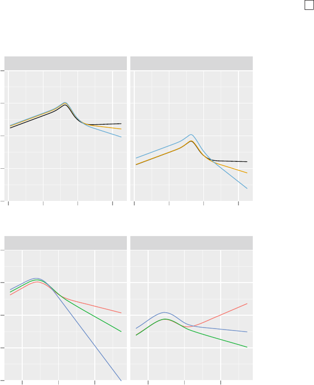
14.10 Using Approximations to Simplify the Model 349

example, the mean absolute error in predicting

L. Another advantage to full

model approximation is that shrinkage used in computing

L is inherited by

any model that predicts

L. In contrast, the usual stepwise methods result in

β that are too large since the ﬁnal coeﬃcients are estimated as if the model

structure were prespeciﬁed. 2

CART would be particularly useful as a model approximator as it would

result in a prediction tree that would be ea sy for health workers to use.

all Y>=1

−3

−2

−1

34 36 38 40 34 36 38 40

Temperature

log odds

all Y>=1

−3

−2

−1

30 60 90 30 60 90

Adjusted respiratory rate

log odds

Fig. 14.7 Centered eﬀects of predictors on the log odds, showing the eﬀects of two

predictors with interaction eﬀects for the age intervals noted. The title all refers

to the prediction of Y =0|Y ≥ 0, that is, Y =0.Y>=1 refers to predicting the

probability of Y =1|Y ≥ 1.

350 14 Ordinal Regression, Data Reduction, and Penalization

Weight−for−age zscore

crying drowsy

feeding hxprob hydration

reffort waz

−1

0.0 2.5 5.0 7.5 10.0 −5 −4 −3 −2 −1 0 1 012345

012345−2 −1 0 1 2.5 5.0 7.5 10.0

012345−4 −2 0 2

log odds

Any Pustular Condition

ausc

bul.conv pustular

−1 0 1

log odds

Fig. 14.8 Centered eﬀects of predictors on the log odds, for predicting Y =1|Y ≥ 1

Unfortunately, a 50-node CART was required to predict

L with an R

≥ 0.9,

and the mean absolute error in the predicted logit was still 0.4. This will

happen when the model contains many important continuous variables.

Let’s approximate the full model using its important components, by using

a step-down technique predicting

L from all of the component variables using

ordinary least squares. In using step-down with the least squares function

ols

in rms there is a problem when the initial R

=1.0 as in that case the esti-

mate of σ = 0. This can be circumvented by specifying an arbitrary nonzero

value of σ to ols (here 1.0), as we are not using the variance–cova riance

matrix from ols anyway. Since cohort interacts with the predictors, separate

approximations can be developed for each level of Y . For this example we

approximate the log odds that Y = 0 using the cohort of patients used fo r

determining Y =0,thatis,Y ≥ 0orcohort=’all’.

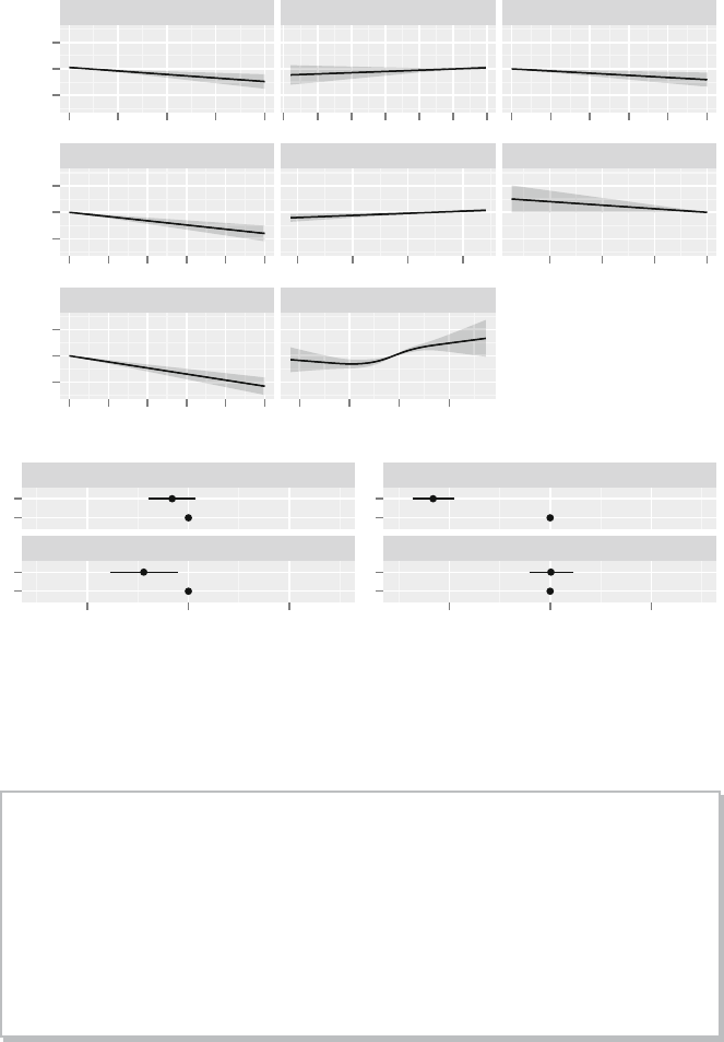
14.10 Using Approximations to Simplify the Model 351

Weight−for−age zscore

crying drowsy

feeding hxprob hydration

reffort waz

−1

0.0 2.5 5.0 7.5 10.0 −5 −4 −3 −2 −1 0 1 012345

012345−2 −1 0 1 2.5 5.0 7.5 10.0

012345−4 −2 0 2

log odds

Any Pustular Condition

ausc

bul.conv pustular

−1 0 1

log odds

Fig. 14.9 Centered eﬀects of predictors on the log odds, for predicting Y ≥ 1. No

plot was made for the fever.ill, stop.breath.orlabor cluster scores.

plogit ← predict(full.pen)

f ← ols(plogit ∼ ageg*(rcs(temp ,5) + rcs(rr ,5)) +

rcs(waz ,4) + bul.conv + drowsy + agitated +

reffort + ausc + feeding + abdominal + hydration +

hxprob + pustular + crying + fever.ill +

stop.breath + labor ,

subset =cohort == ' all ' , data=Sc.expanded , sigma =1)

# Do fast backward stepdown

w ← options(width =120)

fastbw (f, aics=1e10)

352 14 Ordinal Regression, Data Reduction, and Penalization

Deleted Chi−Sq d. f . P Residual d. f . P AIC R2

ageg ∗ temp 1.87 8 0.9848 1.87 8 0.9848 −14.13 1 . 0 0 0

ageg 0.05 2 0.9740 1.92 10 0.9969 −18. 08 1 . 0 0 0

pustular 0.02 1 0.8778 1.94 11 0.9987 −20.06 1 . 0 0 0

fever . i l l 0.08 1 0.7828 2.02 12 0.9994 −21.98 1 . 0 0 0

crying 9.47 1 0.0021 11.49 13 0.5698 −14.51 0 . 9 9 9

abdominal 12.66 1 0.0004 24.15 14 0.0440 −3.85 0.997

rr 17.90 4 0.0013 42.05 18 0.0011 6.05 0.995

hydration 13.21 1 0.0003 55.26 19 0.0000 17.26 0.993

labor 23.48 1 0.0000 78.74 20 0.0000 38.74 0.990

stop . breath 33.40 1 0.0000 112.14 21 0.0000 70.14 0.986

bul . conv 51.53 1 0.0000 163.67 22 0.0000 119.67 0.980

agitated 63.66 1 0.0000 227.33 23 0.0000 181.33 0.972

hxprob 84.16 1 0.0000 311.49 24 0.0000 263.49 0.962

drowsy 109.86 1 0.0000 421.35 25 0.0000 371.35 0.948

temp 295.67 4 0.0000 717.01 29 0.0000 659.01 0.911

waz 368.86 3 0.0000 1085.87 32 0.0000 1021.87 0.866

reff ort 449.83 1 0.0000 1535.70 33 0.0000 1469.70 0.810

ageg ∗ rr 751.19 8 0.0000 2286.90 41 0.0000 2204.90 0.717

ausc 1906.82 1 0.0000 4193.72 42 0.0000 4109.72 0.482

feeding 3900.33 1 0.0000 8094.04 43 0.0000 8008.04 0.000

Approximate E stim ates a f t er D eletin g Facto rs

Coef S . E. Wald Z P

[1 ,] 1.617 0.01482 109.1 0

Factors in Final Model

None

options(w)

# 1e10 causes all variables to eventually be

# deleted so can see most important ones in order

# Fit an approximation to the full penalized model using

# most important variables

full.approx ←

ols(plogit ∼ rcs(temp ,5) + ageg*rcs(rr ,5) +

rcs(waz ,4) + bul.conv + drowsy + reffort +

ausc + feeding ,

subset =cohort == ' all ' , data=Sc.expanded )

p ← predict(full.approx)

abserr ← mean(abs(p - plogit [cohort == ' all ' ]))

Dxy ← somers2(p, y[cohort == ' all ' ])[ ' Dxy ' ]

The approximate model had R

against the full penalized model of 0.972, and

the mean absolute error in predicting

L was 0.17. The D

rank correlation

be tween the approximate model’s predicted logit and the binary event Y =0

14.11 Validating the Model 353

is 0.665 as compared with the full model’s D

=0.672. See Section

19.5 for

an example of computing correct estimates of varia nce of the parameters in

an approximate mo del.

Next turn to diagramming this model approximation so that all predicted

values can be computed without the use of a computer. We draw a type of

nomogram that converts each eﬀect in the model to a 0 to 100 scale which is

just proportional to the log odds. These points are added across predictors

to derive the “Total Points,” which are converted to

L andthentopredicted

probabilities. For the interaction between rr and ageg, rms’s nomogram func-

tion automatically constructs three rr axes—only one is a dded into the total

point score for a given subject. Here we draw a nomogram for predicting the

probability that Y>0, which is 1 − Pr(Y = 0). This probability is derived

by negating

β and X

β in the model derived to predict Pr(Y =0).

f ← full.approx

f$coefficients ← -f$coefficients

f$linear.predictors ← -f$linear.predictors

n ← nomogram(f,

temp=32:41, rr=seq(20,120, by=10),

waz=seq(-1.5 ,2,by=.5),

fun=plogis , funlabel= ' Pr(Y>0) ' ,

fun.at =c(.02 ,.05 ,seq(.1,.9,by=.1),.95 ,.98))

# Print n to see point tables

plot(n, lmgp=.2, cex.axis=.6) # Figure 14.10

newsubject ←

data.frame(ageg= ' [0,7)' , rr=30, temp=39, waz=0, drowsy =5,

reffort=2, bul.conv=0, ausc=0, feeding=0)

xb ← predict(f, newsubject)

The nomogram is shown in Figure 14.10. As an e xample in using the nomo-

gram, a six-day-old infant gets a pproximately 9 points for having a respiration

rate of 30/minute, 19 points for having a temperature of 39

◦

C, 11 points for

waz=0, 14 points for drowsy=5, and 15 points for reffort=2. Assuming that

bul.conv=ausc=feeding=0, that infant gets 68 total points. This corresponds to

β = −0.68 and a probability o f 0.34. 3

14.11 Validating the Model

For the full CR model that was ﬁtted using penalized maximum likelihood

estimation (PMLE), we used 200 bootstrap replications to estimate and then

to correct for optimism in various statistical indexes: D

, generalized R

intercept and slope of a linear r e-calibration equation for X

β,themaximum

calibration error for Pr(Y = 0) based on the linear-logistic re-calibration

(Emax), and the Brier quadratic probability score B.PMLEisusedateach

of the 200 resamples. During the bootstrap simulations, we sample with

354 14 Ordinal Regression, Data Reduction, and Penalization

Points

0 102030405060708090100

Temperature

37 36 35 34 33 32

38 39 41

rr (ageg=[ 0, 7))

40 30 20

50 60 70 90 110

rr (ageg=[ 7,60))

40 30 20

50 60 70 80 90 100 110 120

rr (ageg=[60,90])

40 30 20

50 60 70 80 90 100 110 120

Weight−for−age

zscore

2 1 0 −0.5

bul.conv

drowsy

024

135

reffort

024

135

ausc

feeding

024

135

Total Points

0 20 40 60 80 100 120 140 160 180 200 220 240 260

Linear Predictor

−4 −3 −2 −1 0 1 2 3 4 5 6

Pr(Y>0)

0.02 0.05 0.1 0.2 0.3 0.4 0.5 0.6 0.7 0.8 0.9 0.95 0.98

Fig. 14.10 Nomogram for predicting Pr(Y>0) from the penalized extended CR

model, using an approximate model ﬁtted using ordinary least squares (R

=0.972

against the full model’s predicted logits).

replacement from the patients and not from the 5553 expanded records, hence

the speciﬁcation cluster=u$subs,whereu$subs is the vector of sequential pa-

tient numbers computed from cr.setup ab ove. To be able to assess predictive

accuracy of a sing le predicted probability, the subset parameter is speciﬁed

so that Pr(Y = 0) is being assessed even though 5553 observations are used

to develop each of the 2 00 models.

set.seed(1) # so can reproduce results

v ← validate(full.pen , B=200, cluster=u$subs ,

subset =cohort == ' all ' )

latex(v, file= '', digits =2, size= ' smaller ' )

14.12 Summary 355

Index Original Training Test Optimism Corrected n

Sample Sample Sample Index

0.67 0.68 0.67 0.01 0.66 200

0.38 0.38 0.37 0.01 0.36 200

Intercept −0.03 −0.03 0.00 −0.03 0.00 200

Slope 1.03 1.03 1.00 0. 03 1.00 200

max

0.00 0.00 0.00 0.00 0.00 200

D 0.28 0.29 0.28 0.01 0.27 200

U 0.00 0.00 0.00 0.00 0.00 200

Q 0.28 0.29 0.28 0.01 0. 27 200

B 0.12 0.12 0.12 0.00 0.12 200

g 1.47 1.50 1.45 0.04 1. 42 200

0.22 0.23 0.22 0.00 0.22 200

v ← round (v, 3)

We see that for the apparent D

=0.672 and that the optimism from

overﬁtting was estimated to be 0.011 for the PMLE model, so the bias-

corrected estimate of predictive discrimination is 0.661. The intercept and

slope needed to re-calibrate X

β toa45

◦

line are very near (0, 1). The es-

timate of the maximum calibration error in predicting Pr(Y = 0) is 0.001,

which is quite satisfactory. The corrected Brier score is 0.122.

The simple calibration statistics just listed do not address the issue of

whether predicted values from the model are miscalibrated in a nonlinear

way, so now we estimate an overﬁtting-corrected calibration curve nonpara-

metrically.

cal ← calibrate(full.pen , B=200, cluster=u$subs ,

subset =cohort == ' all ' )

err ← plot(cal) # Figure 14.11

n=5553 Mean a b solute er ror = 0. 0 17 Mean s q ua red e r ror = 0. 00043

0.9 Quantile of absolute error=0.038

The results are shown in Figure 14.11. One can see a slightly nonlinear cali-

bration function estimate, but the overﬁtting-corrected calibration is excellent

everywhere, being only slightly worse than the appa rent calibration. The esti-

mated maximum calibration error is 0.044. The excellent validation for both

predictive discrimination and calibration are a result of the large sample size,

frequency distribution of Y , initial data reduction, and PMLE.

14.12 Summary

Clinically guided variable clustering and item weighting resulted in a great

reduction in the number of candidate predictor degrees of freedom and hence

increased the true predictive accuracy of the model. Scores summarizing clus-

ters of clinical signs, along with temperature, respiration rate, and weight-

for-age after suitable nonlinear transformation and allowance for interactions

356 14 Ordinal Regression, Data Reduction, and Penalization

0.0 0.2 0.4 0.6 0.8 1.0

0.0

0.2

0.4

0.6

0.8

1.0

Predicted Pr{y=1}

Actual Probability

Apparent

Bias−corrected

Ideal

Fig. 14.11 Bootstrap calibration curve for the full penalized extended CR model.

200 bootstrap repetitions were used in conjunction with the loess smoother.

111

Also

shown is a “rug plot” to demonstrate how eﬀective this model is in discriminating

patients into low- and high-risk groups for Pr(Y = 0) (which corresponds with the

derived variable value y =1whencohort=’all’).

with age, are p owerful predictors of the ordinal response. Graphical methods

are eﬀective for detecting lack of ﬁt in the PO and CR models and for dia-

gramming the ﬁnal model. Model approximation allowed development of par-

simonious clinical prediction tools. Appr oximate models inherit the shrinkage

from the full model. For the ordinal model developed here, substantial shrink-

age of the full model was needed.

14.13 Further Reading

See Moons et al.

462

for another case study in penalized maximum likelihood

estimation.

The lasso method of Tibshirani

608,609

also incorporates shrinkage into variable

selection.

To see how this compares with predictions using the full model, the extra clinical

signs in that model that are not in the approximate model were predicted

individually on the basis of X

β from the reduced model along with the signs

that are in that model, using ordinary linear regression. The signs not speciﬁed

when evaluating the approximate model were then set to predicted values based

on the values given for the 6-day-old infant abo ve. The resulting X

β for the full

model is −0.81 and the predicted probability is 0.31, as compared with -0.68

and 0.34 quoted above.

14.14 Problems 357

14.14 Problems

Develop a proportional odds ordinal logistic model predicting the severity

of functional disability (sfdm2) in SUPPORT. The highest level of this vari-

able corresponds to patients dying before the two-month follow-up interviews.

Consider this level as the most severe outcome. Consider the following pre-

dictors: age, sex, dzgroup, num.co, scoma, race (use all levels), meanbp, hrt,

temp, pafi, alb, adlsc. The last variable is the baseline level of functional

disability from the “activities of daily living scale.”

1. For the variables adlsc, sex, age, meanbp, and others if you like, make

plots of means of predictors stratiﬁed by levels of the response, to check

for ordinality. On the same plo t, show estimates of means a ssuming the pro-

portional odds relatio nship b etween predictors and response holds. Com-

ment on the evidence for ordinality and for proportional odds.

2. To allow for maximum adjustment of baseline functional status, treat

this predictor as nominal (after rounding it to the nearest whole num-

be r; fractional values are the result of imputation) in remaining steps, so

that all dummy variables will be generated. Make a single chart showing

proportions of various outcomes stratiﬁed (individually) by

adlsc, sex,

age, meanbp. For continuous predictors use quartiles. You can pass the fol-

lowing function to the summary (summary.formula) function to obtain the

proportions of patients having sfdm2 at or worse than each of its possi-

ble levels (other than the ﬁrst level). An easy way to do this is to use

the cumcategory function with the Hmisc package’s summary.formula func-

tion. cumcategorysummary.formula Print estimates to only two signiﬁcant

digits of precision. Manually check the calculations for the sex variable

using table(sex, sfdm2). Then plot all estimates on a single graph using

plot(object, which=1:4),whereobject was created by summary (actually

summary.formula). Note: for printing tables you may want to convert sfdm2

to a 0–4 variable so that column headers are short and so that later cal-

culations are simpler. You can use for example:

sfdm ← as.integer(sfdm2) - 1

3. Use an R function such as the following to compute the logits of the cu-

mulative proportions.

sf ← function(y)

c( ' Y ≥ 1 ' =qlogis (mean(y ≥ 1)),

' Y ≥ 2 ' =qlogis (mean(y ≥ 2)),

' Y ≥ 3 ' =qlogis (mean(y ≥ 3)),

' Y ≥ 4 ' =qlogis (mean(y ≥ 4)))

As the Y = 3 category is rare, it may be even better to omit the Y ≥ 4

column above, as was done in Section 13.3.9 and Figure 13.1.Foreach

predictor pick two rows of the summary table having reasonable sample

sizes, and take the diﬀerence between the two rows. Comment on the

358 14 Ordinal Regression, Data Reduction, and Penalization

validity o f the proportional odds assumption by assessing how constant

the row diﬀerences are across columns. Note: constant diﬀerences in log

o dds (logits) mean constant ratios of odds or constant relative eﬀects of

the predictor across outcome levels.

4. Make two plots nonparametrically relating age to all of the cumulative

proportions or their logits. You can use commands such as the following

(to use the R Hmisc package).

for(i in 1:4)

plsmo(age , sfdm ≥ i, add=i>1,

ylim=c(.2,.8), ylab= ' Proportion Y ≥ j ' )

for(i in 1:4)

plsmo(age , sfdm ≥ i, add=i>1, fun=qlogis ,

ylim=qlogis (c(.2,.8)), ylab= ' logit ' )

Comment on the linearity of the age eﬀect (which of the two plots do

you use?) and on the proportional odds assumption for age, by a ssessing

parallelism in the second plot.

5. Impute race using the most frequent category and pafi and alb using

“normal” values.

6. Fit a model to predict the ordinal response using all predictors. For con-

tinuous ones a ssume a smooth relationship but allow it to be nonlinear.

Quantify the ability of the model to discriminate patients in the ﬁve out-

comes. Do an overall likelihood ratio test for whether any variables are

associated with the level of functional disability.

7. Compute partial tests of association for each predictor and a test of nonlin-

earity for continuous ones. Compute a global test of nonlinearity. Graphi-

cally display the ranking of importance of the predictors.

8. Display the shape of how each predictor relates to the log odds of exceeding

any level of

sfdm2 you choose, setting other predictors to typical values

(one value per predictor). By default, Predict will make predictions for

the second resp onse category, which is a satisfactory choice here.

9. Use resampling to validate the Somers’ D

rank correlation between pre-

dicted logit and the ordinal outcome. Also validate the generalized R

and slope shrinkage coeﬃcient, all using a single R command. Comment

on the quality (potential “export-ability”) of the model.

Chapter 15

Regression Models for Continuous Y

and Case Study in Ordinal Regression

This chapter concerns univariate continuous Y . There are many multivariable

models for predicting such response variables, such as

• linear mo dels with assumed normal residuals, ﬁtted with ordinary least

squares

• generalized linear models and other parametric models based on special

distributions such as the gamma

• generalized additive models (GAMs)

277

• generalization of GAMs to also nonparametrically transform Y (see

Chapter

16)

• quantile regression (see Section 15.2)

• other robust r egression models that, like quantile regression, use an objec-

tive diﬀerent from minimizing the sum of squared e rrors

635

• semiparametric models based on the ranks of Y , such as the Cox pro-

portional hazards model (Chapter 20) and the proportional odds ordinal

logistic model (Chapters

13 and 14)

• cumulative probability models (often called cumulative link models)which

are semipara metric models from a wider class of families than the logistic.

Semiparametric models that treat Y as ordinal but not interval-scaled have

many advantages including robustness and freedom from all distributional

assumptions for Y conditional on any given set of predictors. Advantages

are demonstrated in a case study of a c umulative probability ordinal model.

Some of the results are compared to quantile regression and OLS. Many of

the methods used in the case study also apply to ordinary linear models.

15.1 The Linear Model

The most popular multivariable model for analyzing a univariate continuous

Y is the linear model

F.E. Harrell, Jr., Regression Modeling Strategies, Springer Series

in Statistics, DOI 10.1007/978-3-319-19425-7

359

360 15 Regression Models for Continuous Y and Case Study in Ordinal Regression

E(Y |X)=Xβ, (15.1)

where β is estimated using ordinary least squares, that is, by solving for

β to

minimize



− X

β)

To compute P -values and conﬁdence limits using parametric methods we

would have to assume that Y |X is normal with mean Xβ and constant vari-

ance σ

. One could estimate conditional means of Y without any distribu-

tional assumptions, but least squares estimators are not robust to outliers or

high-leverage points, and the model would be inaccurate in estimating condi-

tional quantiles of Y |X or Prob[Y ≥ c|X] unless normality of residuals holds.

To be accurate in estimating all quantities, the linear model assumes that

the Gaussian distribution of Y |X

is a simple shift from the distribution of

Y |X

15.2 Quantile Regression

Quantile regression

355, 357

is a diﬀerent approach to modeling Y .Itmakesno

distributional assumptions other than continuity of Y , w hile having all the

usual right hand side assumptions. Quantile regression provides essentially

the same estimates as sa mple quantiles if there is only an intercept or a cate-

gorical predictor in the model. Quantile regression is transformation invariant

— pre-transforming Y is not important.

Quantile regression is a natural generalization of sample quantiles. Let

(y)=y(τ − [y<0]). The τ

sample qua ntile is the minimizer q of



i−1

− q). For a conditional τ

quantile of Y |X the corresponding

quantile regression estimator

minimizes



i=1

− Xβ).

In non-large samples, quantile regression is not as eﬃcient at estimating

quantiles as is ordinary least squares at estimating the mean, if the latter’s

assumptions hold.

Ko enker’s

quantreg package in R

356

implements quantile regression, and

the rms package’s Rq function provides a front-end that gives rise to various

graphics and inference tools.

Using quantile regression, we dir ectly model the median as a function

of cova riates so that only the Xβ structure need be correct. Other quantiles

(e.g., 90

percentile) can be modeled but standard err ors will be much larger

as it is more diﬃcult to pr ecisely estimate outer qua ntiles.

The latter assumption may be dispensed with if we use a robust Huber–White or

bootstrap covariance matrix estimate. Normality may sometimes be dispensed with

by using bootstrap conﬁdence intervals.

15.3 Ordinal Regression Models for Continuous Y 361

15.3 Ordinal Regression Models for Continuous Y

A diﬀerent r obust semiparametric regression approach than quantile regres-

sion is the cumulative probability ordinal model. Semiparametric models

have several advantages over parametric models such as OLS. While quantile

regression has no restriction in the parameters when modeling one quantile

versus another

, ordina l cumulative probability models assume a connection

be tween distributions of Y for diﬀerent X. Ordinal regression even makes

one less assumption than quantile regression about the distribution of Y for

a speciﬁc X: the distribution need not be continuous.

Applying an increasing 1–1 transformation to Y results in no change to

regression coeﬃcient estimates with ordinal regression

. Regression coeﬃcient

estimates are completely robust to extreme Y values

. Estimates of quantiles

of Y from ordinal regression are exactly transformation-preserving, e.g., the

estimate of the median of log Y is exactly the log of the estimate of the

median Y .

For a general continuous distribution function F (y), an ordinal regression

model based on cumulative probabilities may be stated as follows

.Letthe

ordered unique values of Y be denoted by y

,...,y

and let the intercepts

associated with y

,...,y

be α

,α

,...,α

,whereα

= ∞because Prob[Y ≥

]=1.Letα

= α

,i: y

= y.Then

Prob[Y ≥ y

|X]=F (α

+ Xβ)=F (α

+ Xβ) (15.2)

For the OLS fully parametric case, the model may be restated

Prob[Y ≥ y|X]=Prob[

Y − Xβ

≥

y − Xβ

] (15.3)

=1− Φ(

y − Xβ

)=Φ(

−y

Xβ

) (15.4)

Quantile regression allows the estimated value of the 0.5 quantile to be higher than

the estimated value of the 0.6 quantile for some values of X. Composite quantile

regression

690

removes this possibility by forcing all the X coeﬃcients to be the same

across multiple quantiles, a restriction not unlike what cumulative probability ordinal

models make.

For symmetric distributions applying a decreasing transformation will negate the

coeﬃcients. For asymmetric distributions (e.g., Gumbel), reversing the order of Y

will do more than change signs.

Only an estimate of mean Y from these

βs is non-robust.

It is more traditional to state the model in terms of Prob[Y ≤ y|X] but we use

Prob[Y ≥ y|X] so that higher predicted va lues are associated with higher Y .

362 15 Regression Models for Continuous Y and Case Study in Ordinal Regression

Table 15.1 Distribution families used in ordinal cumulative probability models. Φ

denotes the Gaussian cumulative distribution function. For the Connection column,

=Prob[Y ≥ y|X

],P

=Prob[Y ≥ y|X

],Δ =(X

− X

)β. The connection

sp eciﬁes the only distributional assumption if the model is ﬁtted semiparametrically,

i.e, contains an in tercept for every unique Y value less one. For parametric models, P

must be speciﬁed absolutely instead of just requiring a relationship between P

and

. For example, the traditional Gaussian parametric model speciﬁes that Prob[Y ≥

y|X]=1− Φ(

y−Xβ

)=Φ(

−y+Xβ

Distribution F Inverse Link Name Connection

(Link Function)

Logistic [1 + exp(−y)]

−1

log(

1−y

) logit

1−P

exp(∆)

Gaussian Φ(y)

−1

(y)probitP

= Φ(Φ

−1

)+∆)

Gumbel maximum exp(− exp(−y))

log(− log(y)) log − log P

= P

exp(∆)

value

Gumbel minimum 1 − exp(− exp(y)) log(− log(1 − y)) complementary 1 − P

=(1− P

)

exp(∆)

value

log − log

Cauchy

tan

−1

(y)+

tan[π(y −

)] cauchit

so that to within an additive constant

−y

(intercepts α are linear in

y whereas they are arbitrarily descending in the ordinal model), and σ is

absorbed in β to put the OLS model into the new notation.

The genera l ordinal regr e ssion model assumes that for ﬁxed X

−1

(Prob[Y ≥ y|X

]) − F

−1

(Prob[Y ≥ y|X

]) (15.5)

=(X

− X

)β (15.6)

independent of the αs (parallelism assumption). If F =[1+exp(−y)]

−1

,this

is the proportional odds assumption.

Common choices of F , implemented in the R rms orm function, a re shown

in Table

15.1. The Gumbel maximum value distribution is also called the

extreme va lue type I distribution. This distribution (log −log link) also rep-

resents a continuous time proportional hazards model. The hazard ratio when

X changes from X

to X

is exp(−(X

− X

)β).

The mean of Y |X is easily estimated from a ﬁtted cumulative probability

ordinal model by computing



i=1



Prob[Y = y

|X] (15.7)

and the q

quantile of Y |X is y such that F

−1

(1 − q) − X

β =ˆα

ˆα

are unchanged if a constant is added to all y.

The intercepts have to be shifted to the left one position in solving this equation

because the quantile is such that Prob[Y ≤ y]=q whereas the model is stated in

terms of Prob[Y ≥ y].

15.3 Ordinal Regression Models for Continuous Y 363

The orm function in the rms package takes advantage of the information

matrix being of a sparse tri-band diagonal form for the intercept parameters.

This makes the computations eﬃcient even for hundreds of intercepts (i.e.,

unique va lues of Y ). orm is made to handle continuous Y .

Ordinal regression has nice pr operties in addition to those listed above,

allowing for

• estimation of quantiles as eﬃciently as quantile regression if the parallel

slopes assumptions hold

• eﬃcient estimation of mean Y

• direct estimation of Prob[Y ≥ y|X]

• arbitrary clumping of values of Y , while still estimating β and mean Y

eﬃciently

• solutions for

β using ordinary Newton-Raphson or other p opular optimiza-

tion techniques

• b eing based on a standar d likelihood function, penalized estimation can

be straightforward

• Wald, score, and likelihood ratio χ

tests that are more p owerful than tests

from quantile regression.

On the last point, if there is a single predictor in the model a nd it is binary,

the score test from the proportional odds model is essentially the Wilcoxon

test, and the scor e test from the Gumbel log-log cumulative probability

model is essentially the log-rank test.

15.3.1 Minimum Sample Size Requirement

When Y is continuous and the pur pose of an ordinal model includes semi-

parametr ic estimation of probabilities or quantiles, the accuracy of estimates

is limited even more by the accuracy of estimating the empir ical cumulative

distribution of Y than by estimating β.Whenβ = 0, intercept estimates are

transformations of the empirical distribution step function. As described in

Section

20.3, the sample size must be 184 to estimate the entire distribution

of Y with a global margin of error not exceeding 0.1. For estimating the mean

of Y , smaller sample sizes may be needed.

But it is not sensible to estimate quantiles of Y when there are heavy ties in Y in

the area containing the quantile.

364 15 Regression Models for Continuous Y and Case Study in Ordinal Regression

15.4 Comparison of Assumptions of Various Models

Quantile regression makes the fewest left-hand-side model assumptions except

for the assumption that Y be continuo us, but can have less estimator precision

than other models and has lower power. To summarize how assumptions of

parametric models compare to assumptions of semiparametric ordinal models,

consider the ordinary linear model or its sp ecial case the equal variance two-

sample t-test, vs. the probit or logit (proportional odds) ordinal model or

their special cases the Van der Waerden (normal-scores) two-sample rank test

or the Wilcoxon two-sample test. All the assumptions of the linear model

other than independence of residuals are captured in the following, using the

more standard Y ≤ y notation:

F (y |X)=Prob[Y ≤ y|X]=Φ(

y − Xβ

) (15.8)

−1

(F (y|X)) =

y − Xβ

(15.9)

On the other hand, ordinal models assume the following:

−1

(F(y|X))

−ΔXβ σ

−1

(F(y|X))

logit(F(y|X))

−ΔXβ

Fig. 15.1 Assumptions of the linear model (left panel) and semiparametric ordi-

nal probit or logit (proportional odds) models (right panel). Ordinal models do not

assume any shape for the distribution of Y for a given X; they only assume paral-

lelism. The linear model can relax the parallelism assumption if σ is allowed to vary,

but in practice it is diﬃcult to know how to vary it except for the unequal variance

two-sample t-test.

Prob[Y ≤ y|X]=F(g(y) − Xβ), (15.10)

where g is unknown and may be discontinuous. This translates to the paral-

lelism assumption in the right panel of Figure

15.1, whereas the linear model

15.5 Dataset and Descriptive Statistics 365

makes the additional strong assumption of linearity of normal inverse cu-

mulative distribution function, which arises from the Gaussian distributio n

assumption.

15.5 Dataset and Descriptive Statistics

Diabetes Mellitus (DM) type II (adult onset diabetes) is strongly associ-

ated with obesity. The currently b est laboratory test for diab etes measures

glycosylated hemoglobin (HbA

), also called g lycated hemoglobin, glycohe-

moglobin, or hemoglobin A

.HbA

reﬂects average blood glucose for the

preceding 60 to 90 days. HbA

> 7.0 is sometimes taken as a positive di-

agnosis of diabetes even though there are no data to supp ort the use of a

threshold.

The goals of this analyses are to better understand eﬀects of b ody size

measurements on risk of DM and to enhance screening for DM. The best way

to develop a model for DM screening is not to ﬁt a binary logistic model

with HbA

> 7 as the resp onse variable. There are at least two reasons for

this. First, when the rela tionship between a measurement and its ultimate

clinical impact is smooth, all cutpoints are arbitrary. There is no justiﬁcation

for any putative cut on HbA

. Second, such an analysis loses information by

treating HbA

=2 the same as HbA

=6.9, and by treating HbA

=7.1 as

equal to HbA

=10. Failure to use all available information results in larger

standard errors of

β, lower p ower, and wider conﬁdence bands. It is better to

predict continuous HbA

using a continuous response model, then use that

model to estimate the probability that HbA

exceeds any cutoﬀ, or estimate

the 0.9 quantile of HbA

The data used here are from the National Health and Nutrition Examina-

tion Survey (NHANES) 2009–2010 from the U.S. National Center for Health

Statistics/Centers for Disease Control. The original data may be obtained

from

http://www.cdc.gov/nchs/nhanes.htm

; the analysis ﬁle used here,

called nhgh, may be obtained from the DataSets wiki page, along with R code

used to download and create the ﬁle. Note that CDC coded age ≥ 80 as 80.

We use the subset of subjects with age ≥ 21 who have neither been diagnosed

nor treated for DM. Descriptive statistics are shown below.

require(rms)

getHdata (nhgh)

w ← subset(nhgh, age ≥ 21 & dx==0 & tx==0, select=-c(dx,tx))

latex(describe(w), file= '')

366 15 Regression Models for Continuous Y and Case Study in Ordinal Regression

18 Variables 4629 Observations

seqn : Respondent sequence number

n missing unique Info Mean .05 .10 .25 .50 .75 .90 .95

4629 0 4629 1 56902 52136 52633 54284 56930 59495 61079 61641

lowest : 51624 51629 51630 51645 51647

highest: 62152 62153 62155 62157 62158

sex

n missing unique

4629 0 2

male (2259, 49%), female (2370, 51%)

age : Age [years]

n missing unique Info Mean .05 .10 .25 .50 .75 .90 .95

4629 0 703 1 48.57 23.33 26.08 33.92 46.83 61.83 74.83 80.00

lowest : 21.00 21.08 21.17 21.25 21.33

highest: 79.67 79.75 79.83 79.92 80.00

re : Race/Ethnicity

n missing unique

4629 0 5

Mexican American (832, 18%), Other Hispanic (474, 10%)

Non-Hispanic White (2318, 50%), Non-Hispanic Black (756, 16%)

Other Race Including Multi-Racial (249, 5%)

income : Family Income

n missing unique

4389 240 14

[0,5000) (162, 4%), [5000,10000) (216, 5%), [10000,15000) (371, 8%)

[15000,20000) (300, 7%), [20000,25000) (374, 9%)

[25000,35000) (535, 12%), [35000,45000) (421, 10%)

[45000,55000) (346, 8%), [55000,65000) (257, 6%), [65000,75000) (188, 4%)

> 20000 (149, 3%), < 20000 (52, 1%), [75000,100000) (399, 9%)

>= 100000 (619, 14%)

wt : Weight [kg]

n missing unique Info Mean .05 .10 .25 .50 .75 .90 .95

4629 0 890 1 80.49 52.44 57.18 66.10 77.70 91.40 106.52 118.00

lowest : 33.2 36.1 37.9 38.5 38.7

highest: 184.3 186.9 195.3 196.6 203.0

ht : Standing Height [cm]

n missing unique Info Mean .05 .10 .25 .50 .75 .90 .95

4629 0 512 1 167.5 151.1 154.4 160.1 167.2 175.0 181.0 184.8

lowest : 123.3 135.4 137.5 139.4 139.8

highest: 199.2 199.3 199.6 201.7 202.7

15.5 Dataset and Descriptive Statistics 367

bmi : Body Mass Index [kg/m

]

n missing unique Info Mean .05 .10 .25 .50 .75 .90 .95

4629 0 1994 1 28.59 20.02 21.35 24.12 27.60 31.88 36.75 40.68

lowest : 13.18 14.59 15.02 15.40 15.49

highest: 61.20 62.81 65.62 71.30 84.87

leg : Upper Leg Length [cm]

n missing unique Info Mean .05 .10 .25 .50 .75 .90 .95

4474 155 216 1 38.39 32.0 33.5 36.0 38.4 41.0 43.3 44.6

lowest : 20.4 24.9 25.0 25.1 26.4, highest: 49.0 49.5 49.8 50.0 50.3

arml : Upper Arm Length [cm]

n missing unique Info Mean .05 .10 .25 .50 .75 .90 .95

4502 127 156 1 37.01 32.6 33.5 35.0 37.0 39.0 40.6 41.7

lowest : 24.8 27.0 27.5 29.2 29.5, highest: 45.2 45.5 45.6 46.0 47.0

armc : Arm Circumference [cm]

n missing unique Info Mean .05 .10 .25 .50 .75 .90 .95

4499 130 290 1 32.87 25.4 26.9 29.5 32.5 35.8 39.1 41.4

lowest : 17.9 19.0 19.3 19.5 19.9, highest: 54.2 54.9 55.3 56.0 61.0

waist : Waist Circumference [cm]

n missing unique Info Mean .05 .10 .25 .50 .75 .90 .95

4465 164 716 1 97.62 74.8 78.6 86.9 96.3 107.0 117.8 125.0

lowest : 59.7 60.0 61.5 62.0 62.4

highest: 160.0 160.6 162.2 162.7 168.7

tri : Triceps Skinfold [mm]

n missing unique Info Mean .05 .10 .25 .50 .75 .90 .95

4295 334 342 1 18.94 7.2 8.8 12.0 18.0 25.2 31.0 33.8

lowest : 2.6 3.1 3.2 3.3 3.4, highest: 39.6 39.8 40.0 40.2 40.6

sub : Subscapular Skinfold [mm]

n missing unique Info Mean .05 .10 .25 .50 .75 .90 .95

3974 655 329 1 20.8 8.60 10.30 14.40 20.30 26.58 32.00 35.00

lowest : 3.8 4.2 4.6 4.8 4.9, highest: 40.0 40.1 40.2 40.3 40.4

gh : Glycohemoglobin [%]

n missing unique Info Mean .05 .10 .25 .50 .75 .90 .95

4629 0 63 0.99 5.533 4.8 5.0 5.2 5.5 5.8 6.0 6.3

lowest : 4.0 4.1 4.2 4.3 4.4, highest: 11.9 12.0 12.1 12.3 14.5

albumin : Albumin [g/dL]

n missing unique Info Mean .05 .10 .25 .50 .75 .90 .95

4576 53 26 0.99 4.261 3.7 3.9 4.1 4.3 4.5 4.7 4.8

lowest : 2.6 2.7 3.0 3.1 3.2, highest: 4.9 5.0 5.1 5.2 5.3

368 15 Regression Models for Continuous Y and Case Study in Ordinal Regression

bun : Blood urea nitrogen [mg/dL]

n missing unique Info Mean .05 .10 .25 .50 .75 .90 .95

4576 53 50 0.99 13.03 7 8 10 12 15 19 22

lowest : 1 2 3 4 5, highest: 49 53 55 56 63

SCr : Creatinine [mg/dL]

n missing unique Info Mean .05 .10 .25 .50 .75 .90 .95

4576 53 167 1 0.8887 0.58 0.62 0.72 0.84 0.99 1.14 1.25

lowest : 0.34 0.38 0.39 0.40 0.41

highest: 5.98 6.34 9.13 10.98 15.66

dd ← datadist(w); options(datadist= ' dd ' )

15.5.1 Checking Assumptions of OLS

and Other Models

First let’s see if gh would make a Gaussian residuals model ﬁt. Use ordinary

regression on four key variables to collapse these into one variable (predicted

mean from the OLS model). Stratify the pr edicted means into six quantile

groups. Apply the normal inverse cumulative distribution function Φ

−1

to the

empirical cumulative distribution functions (ECDF) of gh using these strata,

and check for normality and constant σ

. The ECDF estimates Prob[Y ≤

y|X] but for ordinal modeling we want to state models in terms of Prob[Y ≥

y|X] so take one minus the ECDF before inverse transforming.

f ← ols (gh ∼ rcs(age ,5) + sex + re + rcs(bmi, 3), data=w)

pgh ← fitted(f)

p ← function (fun, row, col) {

f ← substitute (fun); g ← function (F) eval(f)

z ← Ecdf(∼ gh, groups=cut2(pgh, g=6),

fun=function (F) g(1 - F),

ylab=as.expression(f), xlim=c(4.5, 7.75), data=w,

label.curve =FALSE)

print(z, split=c(col , row , 2, 2), more=row < 2 | col < 2)

}

p(log(F/(1-F)), 1, 1)

p(qnorm(F), 1, 2)

p(-log(-log(F)), 2, 1)

p(log(-log(1-F)), 2, 2)

# Get slopes of pgh for some cutoffs of Y

# Use glm complementary log-log link on Prob(Y < cutoff) to

# get log-log link on Prob(Y ≥ cutoff)

r ← NULL

for(link in c( ' logit ' , ' probit ' , ' cloglog ' ))

for(kinc(5,5.5,6)){

co ← coef(glm(gh < k ∼ pgh , data=w, family=binomial(link)))

15.5 Dataset and Descriptive Statistics 369

r ← rbind(r, data.frame (link=link , cutoff=k,

slope=round(co[2],2)))

}

print(r, row.names =FALSE)

link cutoff slope

logit 5.0 -3.39

logit 5.5 -4.33

logit 6.0 -5.62

probit 5.0 -1.69

probit 5.5 -2.61

probit 6.0 -3.07

cloglog 5.0 -3.18

cloglog 5.5 -2.97

cloglog 6.0 -2.51

Glycohemoglobin, % Glycohemoglobin, %

log(F/(1 − F))

−5

5.0 5.5 6.0 6.5 7.0 7.5

qnorm (F)

−2

5.0 5.5 6.0 6.5 7.0 7.5

− log(− log(F))

−2

5.0 5.5 6.0 6.5 7.0 7.5

log (− log(1 − F))

−6

−4

−2

5.0 5.5 6.0 6.5 7.0 7.5

Fig. 15.2 Examination of normality and constant variance assumption, and assump-

tions for various ordinal models

370 15 Regression Models for Continuous Y and Case Study in Ordinal Regression

The upper right curves in Figure

15.2 are not linear, implying that a normal

conditional distribution cannot work for gh

There is non-parallelism for the

logit model. The other graphs will b e used to guide selection of an ordinal

model below.

15.6 Ordinal Regression Applied to HbA

In the upper left panel of Figure

15.2, logit inverse curves are not parallel

so the proportional odds assumption does not hold when predicting HbA

The log -log link yields the highest degree of parallelism and most constant

regression co eﬃcients across cutoﬀs of gh, so we use this link in an ordinal

regression model (linearity of the curves is not required).

15.6.1 Checking Fit for Various Models Using Age

Another way to examine model ﬁt is to ﬂexibly ﬁt the single most important

predictor (age) using a variety of methods, and compare predictions to sample

quantiles a nd means based on subsets on age . We use overlapping subsets

to gain resolution, with each subset comp osed of those subjects having age

within ﬁve years of the point being predicted by the models. Here we predict

the 0.5, 0.75, and 0.9 quantiles and the mean. For quantiles we can compare

to quantile regression (discussed below) and for means we compare to OLS.

ag ← 25:75

lag ← length(ag)

q2 ← q3 ← p90 ← means ← numeric(lag)

for(i in 1:lag) {

s ← which(abs(w$age - ag[i]) < 5)

y ← w$gh[s]

a ← quantile(y, probs=c(.5, .75, .9))

q2[i] ← a[1]

q3[i] ← a[2]

p90[i] ← a[3]

means[i] ← mean(y)

}

fams ← c( ' logistic ' , ' probit ' , ' loglog ' , ' cloglog ' )

fe ← function(pred , target) mean(abs(pred$yhat - target))

mod ← gh ∼ rcs(age,6)

P ← Er ← list()

for(est in c( ' q2 ' , ' q3 ' , ' p90 ' , ' mean ' )) {

meth ← if(est == ' mean ' ) ' ols ' else ' QR '

p ← list()

er ← rep(NA, 5)

names(er) ← c(fams, meth)

for(family in fams) {

h ← orm(mod, family=family, data=w)

fun ← if(est == ' mean ' ) Mean(h)

else {

qu ← Quantile(h)

They are not parallel either.

15.6 Ordinal Regression Applied to HbA

371

switch(est, q2 = function (x) qu(.5, x),

q3 = function (x) qu(.75, x),

p90 = function (x) qu(.9, x))

}

p[[family]] ← z ← Predict(h, age=ag, fun=fun, conf.int =FALSE)

er[family] ← fe(z, switch(est, mean=means , q2=q2, q3=q3, p90=p90))

}

h ← switch(est,

mean= ols(mod, data=w),

q2 = Rq (mod, data=w),

q3 = Rq (mod, tau=0.75, data=w),

p90 = Rq (mod, tau=0.90, data=w))

p[[meth]] ← z ← Predict(h, age=ag, conf.int =FALSE)

er[meth] ← fe(z, switch(est, mean=means , q2=q2, q3=q3, p90=p90))

Er[[est]] ← er

pr ← do.call( ' rbind ' ,p)

pr$est ← est

P ← rbind.data.frame(P, pr)

}

xyplot(yhat ∼ age | est, groups=.set. , data=P, type= ' l ' , # Figure 15.3

auto.key=list(x=.75, y=.2, points=FALSE , lines=TRUE),

panel=function(..., subscripts) {

panel.xyplot(..., subscripts=subscripts)

est ← P$est[subscripts[1]]

lpoints(ag, switch(est, mean=means , q2=q2, q3=q3, p90=p90),

col=gray(.7))

er ← format(round(Er[[est]],3), nsmall =3)

ltext(26, 6.15, paste(names(er), collapse= ' \n ' ),

cex=.7, adj=0)

ltext(40, 6.15, paste(er, collapse = ' \n ' ),

cex=.7, adj=1)})

It can be seen in Figure 15.3 that models dedicated to a speciﬁc task

(quantile regression for quantiles and OLS for means) were b est for those

tasks. Although the log-log o rdinal cumulative proba bility model did not

estimate the median as accura tely as some other methods, it does well fo r

the 0.75 and 0.9 quantiles and is the best compromise overall because of

its a bility to also directly predict the mean as well as quantities such as

Prob[HbA

> 7|X].

From here on we focus on the log-log ordinal model. Returning to the

bottom left of Figure

15.2, let’s look at quantile groups of predicted HbA

by O LS and plot predicted distr ibutions of actual HbA

against empirical

distributions.

w$pghg ← cut2(pgh , g=6)

f ← orm(gh ∼ pghg , data=w)

lp ← predict (f, newdata=data.frame (pghg=levels(w$pghg)))

ep ← ExProb (f) # Exceedance prob. functn. generator in rms

z ← ep(lp)

j ← order(w$pghg) # puts in order of lp (levels of pghg)

plot(z, xlim=c(4, 7.5), data=w[j,c( ' pghg ' , ' gh ' )]) # Fig. 15.4

Agreement between predicted and observed exceedance probability distribu-

tions is excellent in Figure 15.4.

372 15 Regression Models for Continuous Y and Case Study in Ordinal Regression

age

yhat

5.2

5.4

5.6

5.8

6.0

6.2

30 40 50 60 70

logistic

probit

loglog

cloglog

ols

0.021

0.025

0.026

0.033

0.013

mean

logistic

probit

loglog

cloglog

0.053

0.047

0.041

0.101

0.030

p90

logistic

probit

loglog

cloglog

0.048

0.052

0.058

0.072

0.024

30 40 50 60 70

5.2

5.4

5.6

5.8

6.0

6.2

logistic

probit

loglog

cloglog

0.050

0.045

0.037

0.077

0.027

logistic

probit

loglog

cloglog

ols

Fig. 15.3 Three estimated quantiles and estimated mean using 6 methods, compared

against caliper-matched sample quantiles/means (circles). Numbers are mean abso-

lute diﬀerences between predicted and sample quantities using overlapping intervals

of age and caliper matching. QR:quantile regression.

To return to the initial look a t a linear model with assumed Gaussian

residuals, ﬁt a probit ordinal model and compare the estimated intercepts to

the linear relationship with gh that is assumed by the normal distribution.

f ← orm (gh ∼ rcs(age ,6), family=probit , data=w)

g ← ols (gh ∼ rcs(age ,6), data=w)

s ← g$stats[ ' Sigma ' ]

yu ← f$yunique [-1]

r ← quantile (w$gh, c(.005 , .995))

alphas ← coef(f)[1:num.intercepts(f)]

plot(-yu / s, alphas , type= ' l ' , xlim=rev(- r / s), # Fig. 15.5

xlab=expression (-y/hat(sigma)), ylab=expression (alpha[y]))

Figure 15.5 depicts a signiﬁcant departure from the linear form implied by

Gaussian residuals (Eq.

15.4).

15.6 Ordinal Regression Applied to HbA

373

4.0 4.5 5.0 5.5 6.0 6.5 7.0 7.5

0.0

0.2

0.4

0.6

0.8

1.0

Prob(Y ≥ y)

[4.88,5.29)

[5.29,5.44)

[5.44,5.56)

[5.56,5.66)

[5.66,5.76)

[5.76,6.48]

Fig. 15.4 Observed (dashed lines, open circles) and predicted (solid lines, closed cir-

cles) exceedance probability distributions from a model using 6-tiles of OLS-predicted

HbA

. Key shows quantile group intervals of predicted mean HbA

−14 −12 −10 −8

−5

−4

−3

−2

−1

−y σ

Fig. 15.5 Estimated intercepts from probit mo del. Linearity would have indicated

Gaussian residuals.

374 15 Regression Models for Continuous Y and Case Study in Ordinal Regression

15.6.2 Examination of BMI

Body mass index (BMI, weight divided by height

) is commo nly used as an

obesity measure because it is well correlated with abdominal visceral fat.

But it is not obvious that BMI is the correct summary of height and weight

for predicting pre-clinical diabetes, and it may be the case that body size

measures other than height and weight are better predictors.

Use the log-log ordinal model to check the adequacy of BMI, adjusting for

age (without a ssuming linearity). This can be done by examining the ratio

of coeﬃcients of log height and log weight, and also by using AIC to judge

whether BMI is an adequate summary of height and weight when compared

to nonlinea r functions of the logs, and to a tensor spline interaction surface.

f ← orm(gh ∼ rcs(age,5) + log(ht) + log(wt),

family=loglog, data=w)

print(f, latex=TRUE)

-log-log Ordinal Regression Model

orm(formula = gh ~ rcs(age, 5) + log(ht) + log(wt), data = w,

family = loglog)

Model Likelihood Discrimination Rank Discrim.

Ratio Test Indexes Indexes

Obs 4629 LR χ

1126.94 R

0.217 ρ 0.486

Unique Y 63 d.f. 6 g 0.627

0.5

5.5 Pr(>χ

) < 0.0001 g

1.872

max |

∂ log L

∂β

Score χ

1262.81 |Pr(Y ≥ Y

0.5

) −

| 0.153

1×10

−6

Pr(>χ

) < 0.0001

Coef S.E. Wald Z Pr(> |Z|)

age 0.0398 0.0055 7.29 < 0.0001

age’ -0.0158 0.0275 -0.57 0.5657

age” -0.0072 0.0866 -0.08 0.9333

age”’ 0.0309 0.1135 0.27 0.7853

ht -3.0680 0.2789 -11.00 < 0.0001

wt 1.2748 0.0704 18.10 < 0.0001

aic ← NULL

for(mod in list(gh ∼ rcs(age ,5) + rcs(log(bmi),5),

gh ∼ rcs(age ,5) + rcs(log(ht),5) + rcs(log(wt),5),

gh ∼ rcs(age ,5) + rcs(log(ht),4) * rcs(log(wt),4)))

aic ← c(aic, AIC(orm(mod, family=loglog, data=w)))

print(aic)

[1] 25910.77 25910.17 25906.03

15.6 Ordinal Regression Applied to HbA

375

The ratio of the coeﬃcient of log height to the co eﬃcient of log weight is -

2.4, which is between what BMI uses and the more dimensionally reasonable

weight / height

. By AIC, a spline interaction surface between height and

weight does slightly better than BMI in predicting HbA

, but a nonlinear

function of BMI is barely worse. It will require other body size measures to

displace BMI as a predictor.

As an aside, compare this model ﬁt to that from the Cox proportional

hazards model. The Cox model uses a conditioning argument to obtain

a partial likelihood free of the intercepts α (and requires a second step to

estimate these log discrete hazard components) whereas we are using a full

marginal likelihood of the ranks of Y

330

print(cph(Surv(gh) ∼ rcs(age,5) + log(ht) + log(wt), data=w),

latex=TRUE)

Cox Proportional Hazards Model

cph(formula = Surv(gh) ~ rcs(age, 5) + log(ht)

+ log(wt), data = w)

Model Tests Discrimination

Indexes

Obs 4629 LR χ

1120.20 R

0.215

Events 4629 d.f. 6 D

0.359

Center 8.3792 Pr(>χ

) 0.0000 g 0.622

Score χ

1258.07 g

1.863

Pr(>χ

) 0.0000

Coef S.E. Wald Z Pr(> |Z|)

age -0.0392 0.0054 -7.24 < 0.0001

age’ 0.0148 0.0274 0.54 0.5888

age” 0.0093 0.0862 0.11 0.9144

age”’ -0.0321 0.1131 -0.28 0.7767

ht 3.0477 0.2779 10.97 < 0.0001

wt -1.2653 0.0701 -18.04 < 0.0001

Close agreement of the two is seen, as expected.

15.6.3 Consideration of All Body Size Measurements

Next we examine all body size mea sures, and check their r edundancies.

v ← varclus(∼ wt + ht + bmi + leg + arml + armc + waist +

tri + sub + age + sex + re, data=w)

plot(v)

376 15 Regression Models for Continuous Y and Case Study in Ordinal Regression

# Omit wt so it won ' t be removed before bmi

redun(∼ ht + bmi + leg + arml + armc + waist + tri + sub ,

data=w, r2=.75)

Redundancy Analysis

redun(formula = ∼ht + bmi + leg + arml + armc + waist + tri +

sub, data = w, r2 = 0.75)

n: 3853 p: 8 nk: 3

Number of NAs: 776

Frequencies of Missing Values Due to Each Variable

ht bmi leg arml armc waist tri sub

0 0 155 127 130 164 334 655

Transformation of target variables forced to be linear

cutoff: 0.75 Type: ordinary

with which each variable can be predicted from all other variables:

ht bmi leg arml armc waist tri sub

0.829 0.924 0.682 0.748 0.843 0.864 0.531 0.594

Rendundant variables:

bmi ht

Predicted from variables:

leg arml armc waist tri sub

Variable Deleted R

after later deletions

1 bmi 0.924 0.909

2 ht 0.792

Six size measures adequately capture the entire set. Height a nd BMI are

removed (Figure 15.6). An advantage of removing height is that it is age-

dependent due to vertebral compression in the elderly:

f ← orm(ht ∼ rcs(age ,4)*sex , data=w) # Prop. odds model

qu ← Quantile(f); med ← function(x) qu(.5, x)

ggplot (Predict(f, age , sex , fun=med , conf.int=FALSE),

ylab= ' Predicted Median Height , cm ' )

However, upper leg length has the same declining tr end, implying a survival

bias or birth year eﬀect.

In preparing to create a multivariable model, degrees of freedom are allo-

cated according to the generalized Spearman ρ

(Figure

15.7)

s ← spearman2(gh ∼ age + sex + re + wt + leg + arml + armc +

waist + tri + sub , data=w, p=2)

plot(s)

Parameters will be allocated in descending order of ρ

. But note that

subscapular skinfold has a large number o f NAs and other predictors also have

NAs. Suboptimal casewise deletion will be used until the ﬁnal model is ﬁtted

(Figure

15.8).

Competition between collinear size measures hurts interpretation of partial tests of

association in a saturated additive model.

15.6 Ordinal Regression Applied to HbA

377

bmi

waist

armc

tri

sub

sexfemale

leg

arml

age

reOther Race Including Multi−Racial

reOther Hispanic

reNon−Hispanic White

reNon−Hispanic Black

1.0

0.8

0.6

0.4

0.2

0.0

Spearman ρ

Fig. 15.6 Variable clustering for all potential predictors

155

160

165

170

175

180

20 40 60 80

Age, years

Predicted Median Height, cm

sex

male

female

Fig. 15.7 Estimated median height as a smooth function of age, allowing age to

interact with sex, from a proportional odds model

Because there are many competing body measures, we use backwards step-

down to arrive at a set of predictors. The bootstrap will be used to pe nal-

ize predictive ability for variable selection. First the full model is ﬁt using

casewise deletion, then we do a composite test to assess whether any of the

frequently–missing predictors is important.

f ← orm(gh ∼ rcs(age,5) + sex + re + rcs(wt,3) + rcs(leg,3) + arml +

rcs(armc ,3) + rcs(waist ,4) + tri + rcs(sub ,3),

family= ' loglog ' , data=w, x=TRUE , y=TRUE)

print(f, latex=TRUE , coefs=FALSE)

378 15 Regression Models for Continuous Y and Case Study in Ordinal Regression

age

waist

leg

sub

armc

tri

arml

sex

N df

4629 1

4502 2

4295 2

4629 4

4629 2

4499 2

3974 2

4474 2

4465 2

4629 2

0.00 0.05 0.10 0.15 0.20

Spearman ρ

Response : gh

Adjusted ρ

Fig. 15.8 Generalized squared rank correlations

-log-log Ordinal Regression Model

orm(formula = gh ~ rcs(age, 5) + sex + re + rcs(wt, 3)

+ rcs(leg, 3) + arml + rcs(armc, 3) + rcs(waist, 4)

+ tri + rcs(sub, 3), data = w, x = TRUE, y = TRUE,

family = "loglog")

Frequencies of Missing Values Due to Each Variable

0 100 200 300 400 500 600 700

655

334

164

155

130

127

sub

tri

waist

leg

armc

arml

age

sex

15.6 Ordinal Regression Applied to HbA

379

Model Likelihood Discrimination Rank Discrim.

Ratio Test Indexes Indexes

Obs 3853 LR χ

1180.13 R

0.265 ρ 0.520

Unique Y 60 d.f. 22 g 0.732

0.5

5.5 Pr(>χ

) < 0.0001 g

2.080

max |

∂ log L

∂β

Score χ

1298.88 |Pr(Y ≥ Y

0.5

) −

| 0.172

3×10

−5

Pr(>χ

) < 0.0001

## Composite test :

lan ← function(a) latex(a, table.env=FALSE , file= '')

lan(anova(f, leg, arml , armc , waist , tri , sub))

d.f. P

leg 8.30 2 0.0158

Nonlinear 3.32 1 0.0685

arml 0.16 1 0.6924

armc 6.66 2 0.0358

Nonlinear 3.29 1 0.0695

waist 29 .40 3 < 0.0001

Nonlinear 4.29 2 0.1171

tri 16.62 1 < 0.0001

sub 40.75 2 < 0.0001

Nonlinear 4.50 1 0.0340

TOTAL NONLINEAR 14.95 5 0.0106

TOTAL 128.29 11 < 0.0001

The model achieves Spearman ρ =0.52, the r ank correlation between

predicted and observed HbA

We show the predicted mean and median HbA

as a function of age,

adjusting other variables to their median or mode (Figure

15.9). Compare the

estimate of the median and 90

percentile with that from quantile regression.

M ← Mean(f)

qu ← Quantile(f)

med ← function(x) qu(.5, x)

p90 ← function(x) qu(.9, x)

fq ← Rq(formula(f), data=w)

fq90 ← Rq(formula(f), data=w, tau=.9)

pmean ← Predict(f, age , fun=M, conf.int=FALSE)

pmed ← Predict(f, age , fun=med , conf.int=FALSE)

p90 ← Predict(f, age , fun=p90 , conf.int=FALSE)

pmedqr ← Predict(fq, age , conf.int=FALSE)

p90qr ← Predict(fq90 , age , conf.int=FALSE)

z ← rbind ( ' orm mean ' =pmean , ' orm median ' =pmed , ' orm P90 ' =p90 ,

' QR median ' =pmedqr , ' QR P90 ' =p90qr)

ggplot (z, groups = ' .set. ' ,

adj.subtitle =FALSE , legend.label =FALSE )

380 15 Regression Models for Continuous Y and Case Study in Ordinal Regression

print(fastbw (f, rule= ' p ' ), estimates=FALSE)

5.00

5.25

5.50

5.75

6.00

20 40 60 80

Age, years

orm mean

orm median

orm P90

QR median

QR P90

Fig. 15.9 Estimated mean and 0.5 and 0.9 quantiles from the log-log ordinal model

using casewise deletion, along with predictions of 0.5 and 0.9 quantiles from quantile

regression (QR). Age is varied and other predictors are held constant to medians/-

modes.

Deleted Chi-Sq d.f. P Residual d.f. P AIC

arml 0.16 1 0.6924 0.16 1 0.6924 -1.84

sex 0.45 1 0.5019 0.61 2 0.7381 -3.39

wt 5.72 2 0.0572 6.33 4 0.1759 -1.67

armc 3.32 2 0.1897 9.65 6 0.1400 -2.35

Factors in Final Model

[1] age re leg waist tri sub

set.seed(13) # so can reproduce results

v ← validate(f, B=100, bw=TRUE , estimates=FALSE , rule= ' p ' )

15.6 Ordinal Regression Applied to HbA

381

Backwards Step-down - Original Model

Deleted Chi-Sq d.f. P Residual d.f. P AIC

arml 0.16 1 0.6924 0.16 1 0.6924 -1.84

sex 0.45 1 0.5019 0.61 2 0.7381 -3.39

wt 5.72 2 0.0572 6.33 4 0.1759 -1.67

armc 3.32 2 0.1897 9.65 6 0.1400 -2.35

Factors in Final Model

[1] age re leg waist tri sub

# Show number of variables selected in first 30 boots

latex(v, B=30, file= '', size= ' small ' )

Index Original Training Test Optimism Corrected n

Sample Sample Sample Index

ρ 0.5225 0.5290 0.5208 0.0083 0.5142 100

0.2712 0.2788 0.2692 0. 0095 0.2617 100

Slope 1.0000 1.0000 0.9761 0.0239 0.9761 100

g 1.2276 1.2505 1.2207 0. 0298 1.1978 100

Pr(Y ≥ Y

0.5

) −

| 0.2007 0.2050 0.1987 0.0064 0.1943 100

Factors Retained in Backwards Elimination

First 30 Resamples

age sex re wt leg arml armc waist tri sub

••••• • • •

••• ••••

••••• • • •

••• ••••

•••• • • •

••••• • •

•••• ••••

••••• • • •

••• ••••

••••••••

•••• ••••

••• ••••

•••• ••••

••••• • • ••

••• •••

•••• ••••

••• ••••

•••• ••••

••• • • •

••• • ••

•••• ••••

••• ••••

•••• ••••

••• • ••

382 15 Regression Models for Continuous Y and Case Study in Ordinal Regression

Frequencies of Numbers of Factors Retained

5678910

11929464 1

Next we ﬁt the reduced model, using multiple imputation to impute miss-

ing predictors (Figure 15.10).

a ← aregImpute(∼ gh + wt + ht + bmi + leg + arml + armc + waist +

tri + sub + age +re, data=w, n.impute =5, pr=FALSE)

g ← fit.mult.impute(gh ∼ rcs(age,5) + re + rcs(leg,3) +

rcs(waist ,4) + tri + rcs(sub ,4),

orm, a, family=loglog, data=w, pr=FALSE)

print(g, latex=TRUE , needspace= ' 1.5in ' )

-log-log Ordinal Regression Model

fit.mult.impute(formula = gh ~ rcs(age, 5) + re + rcs(leg, 3)

+ rcs(waist, 4) + tri + rcs(sub, 4), fitter = orm,

xtrans = a, data = w, pr = FALSE, family = loglog)

Model Likelihood Discrimination Rank Discrim.

Ratio Test Indexes Indexes

Obs 4629 LR χ

1448.42 R

0.269 ρ 0.513

Unique Y 63 d.f. 17 g 0.743

0.5

5.5 Pr(>χ

) < 0.0001 g

2.102

max |

∂ log L

∂β

Score χ

1569.21 |Pr(Y ≥ Y

0.5

) −

| 0.173

1×10

−5

Pr(>χ

) < 0.0001

Coef S.E. Wald Z Pr(> |Z|)

age 0.0404 0.0055 7.29 < 0.0001

age’ -0.0228 0.0279 -0.82 0.4137

age” 0.0126 0.0876 0.14 0.8857

age”’ 0.0424 0.1148 0.37 0.7116

re=Other Hispanic -0.0766 0.0597 -1.28 0.1992

re=Non-Hispanic White -0.4121 0.0449 -9.17 < 0.0001

re=Non-Hispanic Black 0.0645 0.0566 1.14 0.2543

re=Other Race Including Multi-Racial -0.0555 0.0750 -0.74 0.4593

leg -0.0339 0.0091 -3.73 0.0002

leg’ 0.0153 0.0105 1.46 0.1434

waist 0.0073 0.0050 1.47 0.1428

waist’ 0.0304 0.0158 1.93 0.0536

waist” -0.0910 0.0508 -1.79 0.0732

tri -0.0163 0.0026 -6.28 < 0.0001

sub -0.0027 0.0097 -0.28 0.7817

sub’ 0.0674 0.0289 2.33 0.0198

sub” -0.1895 0.0922 -2.06 0.0398

15.6 Ordinal Regression Applied to HbA

383

an ← anova(g)

lan(an)

d.f. P

age 692.50 4 < 0.0001

Nonlinear 28.47 3 < 0.0001

re 168.91 4 < 0.0001

leg 24.37 2 < 0.0001

Nonlinear 2.14 1 0.1434

waist 128.31 3 < 0.0001

Nonlinear 4.05 2 0.1318

tri 39.44 1 < 0.0001

sub 39.30 3 < 0.0001

Nonlinear 6.63 2 0.0363

TOTAL NONLINEAR 46.80 8 < 0.0001

TOTAL 1464.24 17 < 0.0001

b ← anova(g, leg, waist , tri, sub)

# Add new lines to the plot with combined effect of 4 size var.

s ← rbind(an, size=b[ ' TOTAL ' ,])

class(s) ← ' anova.rms'

plot(s)

leg

sub

tri

waist

size

age

0 100 200 300 400 500 600 700

− df

Fig. 15.10 ANOVA for reduced model, after multiple imputation, with addition of

a combined eﬀect for four size variables

ggplot(Predict(g), abbrev=TRUE, ylab=NULL) # Figure 15.11

384 15 Regression Models for Continuous Y and Case Study in Ordinal Regression

Compare the estimated age partial eﬀects and conﬁdence intervals with

those from a model using casewise deletion, and with bootstrap nonparamet-

ric conﬁdence intervals (also with casewise deletio n).

−1.0

−0.5

0.0

0.5

1.0

1.5

20 40 60 80

Age, years

−1.0

−0.5

0.0

0.5

1.0

1.5

30 35 40 45

Upper Leg Length, cm

MxcnAm

OthrHs

Nn−HsW

Nn−HsB

ORIM−R

−1.0−0.50.0 0.5 1.0 1.5

Race Ethnicity

−1.0

−0.5

0.0

0.5

1.0

1.5

10 20 30 40

Subscapular Skinfold, mm

−1.0

−0.5

0.0

0.5

1.0

1.5

10 20 30 40

Triceps Skinfold, mm

−1.0

−0.5

0.0

0.5

1.0

1.5

80 100 120 140

Waist Circumference, cm

Fig. 15.11 Partial eﬀects (log hazard or log-log cumulative probability scale) of all

predictors in reduced model, after multiple imputation

gc ← orm(gh ∼ rcs(age ,5) + re + rcs(leg ,3) +

rcs(waist ,4) + tri + rcs(sub ,4),

family =loglog , data=w, x=TRUE , y=TRUE)

gb ← bootcov(gc, B=300)

bootclb ← Predict(gb, age , boot.type= ' basic ' )

bootclp ← Predict(gb, age , boot.type= ' percentile ' )

multimp ← Predict(g, age)

plot(Predict(gc, age), addpanel=function(...) {

with(bootclb , {llines (age , lower , col= ' blue ' )

llines (age , upper , col= ' blue ' )})

with(bootclp , {llines (age , lower , col= ' blue ' , lty=2)

llines (age , upper , col= ' blue ' , lty =2)})

with(multimp , {llines (age , lower , col= ' red ' )

llines (age , upper , col= ' red ' )

llines (age , yhat , col= ' red ' )} ) },

col.fill=gray(.9), adj.subtitle =FALSE) # Figure 15.12

15.6 Ordinal Regression Applied to HbA

385

Age, years

log hazard

−0.5

0.0

0.5

1.0

20 30 40 50 60 70 80

Fig. 15.12 Partial eﬀect for age from multiple imputation (center red line) and

casewise deletion (center blue line) with symmetric Wald 0.95 conﬁdence bands using

casewise deletion (gray shaded area), basic bootstrap conﬁdence bands using casewise

deletion (blue lines), p ercentile bootstrap conﬁdence bands using casewise deletion

(dashed blue lines), and symmetric Wald conﬁdence bands accounting for multiple

imputation (red lines).

Figure

15.13 depicts the relationship between various predicted quantities,

demonstrating that the ordinal model makes fewer model assumptions that

dictate their connections. A Gaussian or log-Gaussian model would have a

straight-line relationship b etween the predicted mean and median.

M ← Mean(g)

qu ← Quantile(g)

med ← function(lp) qu(.5, lp)

q90 ← function(lp) qu(.9, lp)

lp ← predict(g)

lpr ← quantile(predict(g), c(.002 , .998), na.rm=TRUE)

lps ← seq(lpr[1], lpr[2], length =200)

pmn ← M(lps)

pme ← med(lps)

p90 ← q90(lps)

plot(pmn , pme , # Figure 15.13

xlab=expression (paste( ' Predicted Mean ' , HbA["1c"])),

ylab= ' Median and 0.9 Quantile ' , type= ' l ' ,

xlim=c(4.75 , 8.0), ylim=c(4.75 , 8.0), bty= ' n ' )

box(col=gray(.8))

386 15 Regression Models for Continuous Y and Case Study in Ordinal Regression

lines(pmn , p90 , col= ' blue ' )

abline (a=0, b=1, col=gray(.8))

text(6.5, 5.5, ' Median ' )

text(5.5, 6.3, ' 0.9 ' , col= ' blue ' )

nint ← 350

scat1d (M(lp), nint=nint)

scat1d (med(lp), side=2, nint=nint)

scat1d (q90(lp), side=4, col= ' blue ' , nint=nint)

5.0 5.5 6.0 6.5 7.0 7.5 8.0

5.0

5.5

6.0

6.5

7.0

7.5

8.0

Predicted Mean HbA

Median and 0.9 Quantile

Median

0.9

Fig. 15.13 Predicted mean HbA

vs. predicted median and 0.9 quantile along with

their marginal distributions

Finally, let us draw a nomogram that shows the full power of o rdinal

models, by predicting ﬁve quantities of interest.

g ← Newlevels(g, list(re=abbreviate (levels (w$re))))

exprob ← ExProb (g)

nom ←

nomogram(g, fun=list(Mean=M,

' Median Glycohemoglobin ' = med ,

' 0.9 Quantile ' = q90 ,

' Prob(HbA1c ≥ 6.5) ' =

function(x) exprob (x, y=6.5),

' Prob(HbA1c ≥ 7.0) ' =

function(x) exprob (x, y=7),

' Prob(HbA1c ≥ 7.5) ' =

15.6 Ordinal Regression Applied to HbA

387

function(x) exprob (x, y=7.5)),

fun.at =list(seq(5, 8, by=.5),

c(5,5.25 ,5.5 ,5.75 ,6,6 .25),

c(5.5,6,6.5 ,7,8,10,12,14),

c(.01 ,.05 ,.1,.2,.3,.4),

c(.01 ,.05 ,.1,.2,.3,.4 )))

plot(nom , lmgp=.28) # Figure 15.14

Points

0 102030405060708090100

20 25 30 35 40 45 50 55 60 65 70 75 80

Race/Ethnicity

N−HW ORIM

OthH

Upper Leg Length

55 45 35 30 25 20

Waist Circumference

50 70 90 100 110 120 130 140 150 160 170

Triceps Skinfold

45 35 25 15 5 0

Subscapular Skinfold

15 20 25 30 35 40 45

Total Points

0 20 40 60 80 100 120 140 160 180 200 220 240 260 280

Linear Predictor

−1.5 −1 −0.5 0 0.5 1 1.5 2 2.5

Mean

5 5.5 6 6.5 7 7.5 8

Median Glycohemoglobin

5 5.25 5.5 5.75 6 6.25

0.9 Quantile

5.5 6 6.5 7 8 10 12 14

Prob(HbA1c >= 6.5)

0.01 0.05 0.1 0.2 0.3 0.4

Prob(HbA1c >= 7.0)

0.01 0.05 0.1 0.2 0.3 0.4

Prob(HbA1c >= 7.5)

0.01 0.05 0.1 0.2 0.3

Fig. 15.14 Nomogram for predicting median, mean, and 0.9 quantile of glycohe-

moglobin, along with the estimated probability that HbA

≥ 6.5, 7, or 7.5, all from

the log-log ordinal model

Chapter 16

Transform-Both-Sides Regression

16.1 Background

Fitting multiple regression models by the method of least squares is one of the

most commonly used methods in statistics. There are a number of challenges

to the use of least squares, even when it is only used for estimation and not

inference, including the following.

1. How should continuous predictors be transformed so as to get a good ﬁt?

2. Is it better to transform the response variable? How does one ﬁnd a good

transformation that simpliﬁes the right-hand side of the equation?

3. What if Y needs to be transformed non-monotonically (e.g., |Y − 100|)

before it will have any correlation with X?

When one is trying to draw an inference about population eﬀects using con-

ﬁdence limits or hypothesis tests, the most common approach is to assume

that the residuals have a normal distribution. This is equivalent to assuming

that the conditional distribution of the response Y given the set of predictors

X is normal with mean depending on X and variance that is (one hop es)

a constant independent of X. The need for a distributional assumption to

enable us to draw inferences creates a number of other challenges such as the

following.

1. If for the untransformed original scale of the response Y the distribution of

the residuals is not normal with constant spread, ordinary methods will not

yield correct inferences (e.g., conﬁdence intervals will not have the desired

coverage probability and the intervals will need to b e asymmetric).

2. Quite often there is a transformation of Y that will yield well-behaving

residuals. How do you ﬁnd this transformation? Can you ﬁnd a transfor-

mation for the Xs at the same time?

F.E. Harrell, Jr., Regression Modeling Strategies, Springer Series

in Statistics, DOI 10.1007/978-3-319-19425-7

389

390 16 Transform-Both-Sides Regression

3. All classical statistical inferential methods assume that the full model was

pre-speciﬁed, that is, the model was not modiﬁed after examining the data.

How does one correct conﬁdence limits, for example, for data-based model

and transformation selection?

16.2 Generalized Additive Models

Hastie and Tibshirani

275

have developed generalized additive models (GAMs)

for a variety of distributions for Y . There are semiparametric GAMs, but

most GAMs for continuous Y assume that the conditional distribution of Y is

from a s peciﬁc distribution family. GAMs nicely estimate the transformation

each continuous X requires so as to optimize a ﬁtting criterion s uch as sum

of squared errors or log likelihood, subject to the degrees of freedom the

analyst desires to spend on each predictor. However, GAMs assume that Y

has already been transformed to ﬁt the speciﬁed distr ibution family.

There is excellent software available for ﬁtting a wide variety of GAMs,

such as the

R packages gam, mgcv,androbustgam.

16.3 Nonparametric Estimation of Y -Transformation

When the model’s left-hand side also needs transformation, either to im-

prove R

or to achieve co nstant variance of the residuals (which increases the

chances of satisfying a normality assumption), there are a few approaches

available. One approach is Breiman and Friedman’s alternating conditional

expectation (ACE) method.

ACE simultaneously transforms both Y and

each of the Xs so as to maximize the multiple R

between the transformed

Y and the transformed Xs. The model is given by

g(Y )=f

)+f

)+...+ f

). (16.1)

ACE allows the analyst to impose restrictions on the transformations such

as monotonicity. It allows for categorical predictors, whose categories will

automatically be given numeric scores. The transformation for Y is allowed to

be non-monotonic. One feature of ACE is its ability to estimate the maximal

correlation between an X and the response Y . Unlike the ordinary correlation

co eﬃcient (which assumes linearity) or Spearman’s rank correlation (which

assumes monotonicity), the maximal correlation has the prop erty that it is

zero if and only if X and Y are statistically independent. This property holds

because ACE allows for non-monotonic transformations of all variables. The

“super smoother”(see the S

supsmu function) is the basis for the nonparametric

estimation of transformations for continuous Xs.

16.4 Obtaining Estimates on the Original Scale 391

Tibshirani developed a diﬀerent algorithm for nonparametric additive

regression based on least squares, additivity and varianc e stabilization

(AVAS) .

607

Unlike ACE, AVAS forces g(Y ) to be monotonic. AVAS’s ﬁt-

ting criterion is to maximize R

while forcing the transformation for Y to

result in near ly constant variance of residua ls. The model speciﬁcation is the

same as for ACE (Equation

16.3).

ACE and AVAS are powerful ﬁtting algor ithms, but they can result in over-

ﬁtting (R

can be greatly inﬂated when o ne ﬁts many predictors), and they

provide no statistical inferential measures. As discussed earlier, the process of

estimating transformations (especially those for Y ) can result in signiﬁcant

variance under-estimation, especially for small sample sizes. The boo tstrap

can be used to correct the apparent R

app

) for overﬁtting. As before,

it estimates the optimism (bias) in R

app

and subtracts this optimism from

app

to get a more trustworthy estimate. The bootstr ap can also be used to

compute conﬁdence limits for all estimated transformations, and conﬁdence

limits for estimated predictor eﬀects that take fully into account the uncer-

tainty associated with the transformations. To do this, all steps involved in

ﬁtting the additive models must be re peated fresh for each re-sample.

Limited testing has shown that the sample size needs to exceed 100 for

ACE and AVAS to provide stable estimates. In small sample sizes the boot-

strap bias-corrected estimate of R

will be zero because the sample informa-

tion did not support simultaneous estimation of all transformations.

16.4 Obtaining Estimates on the Original Scale

A common practice in least squar es ﬁtting is to attempt to rectify lack of

ﬁt by taking parametric transformations of Y before ﬁtting; the logarithm

is the most common transformation.

If after transformation the model’s

residuals have a population median of zero, the inverse transformation of a

predicted transformed va lue estimates the population median of Y given X.

This is because unlike means, quantiles are transformation-preserving. Many

analysts make the mistake of not reporting which population parameter is

be ing estimated when inverse transforming X

β, and sometimes they even

report that the mea n is b eing estimated.

How would one go about estimating the population mean or other param-

eter on the untransformed scale? If the residuals are assumed to b e normally

distributed and if log(Y ) is the transformation, the mean of the log-normal

distribution, a function of both the mean and the variance of the residuals,

can be used to derive the desired quantity. However, if the r esiduals are not

normally distributed, this procedure will not result in the correct estimator.

A disadvantage of transform-both-sides regression is this diﬃculty of interpreting

estimates on the original scale. Sometimes the use of a special generalized linear model

can allow for a good ﬁt without transforming Y .

392 16 Transform-Both-Sides Regression

Duan

165

developed a “smearing” estimator for more nonparametrically ob-

taining estimates of parameters on the original scale. In the simple one-sample

case without predictors in which o ne has computed

θ =



i=1

log(Y

)/n,the

residuals from this ﬁtted value are given by e

= log(Y

) −

θ. The smearing

estimator of the population mean is



exp[

θ + e

]/n. In this simple case the

result is the ordinary sample mean

Y .

The worth o f Duan’s smearing estimator is in regression modeling. Sup-

pose that the regression was run on g(Y ) from which estimated values

ˆg(Y

)=X

β and residuals on the transformed scale e

=ˆg(Y

)−X

β were ob-

tained. Instead of restricting ourselves to estimating the population mean, let

W (y

,...,y

) denote any function of a vector of untransformed response

values. To estimate the population mean in the homogeneous one-sample

case, W is the simple average of all of its arguments. To estimate the pop-

ulation 0.25 quantile, W is the sample 0.25 quantile of y

,...,y

. Then the

smearing estimator of the population parameter estimated by W given X is

W (g

−1

(a + e

),g

−1

(a + e

),...,g

−1

(a + e

)), where g

−1

is the inverse of the

g transformation and a = X

β.

When using the AVAS algorithm, the monotonic transformation g is es-

timated from the data, and the predicted value of ˆg(Y ) is given by Equa-

tion

16.3. So we extend the smearing estimator as W (ˆg

−1

(a+e

),...,ˆg

−1

(a+

)), where a is the predicted transformed response given X.Asˆg is non-

parametric (i.e., a table look-up), the areg.boot function described below

computes ˆg

−1

using reverse linear interpolation.

If residuals from ˆg(Y ) are assumed to be symmetrica lly distributed, their

population median is zero and we can estimate the median on the untrans-

formed scale by computing ˆg

−1

β). To be safe, areg.boot adds the median

residual to X

β when estimating the population median (the median r esidual

can be ignored by specifying statistic=’fitted’ to functions that operate on

objects created by areg.boot).

When quantiles of Y are of major interest, a more direct way to obtain

estimates is through the use of quantile regression

357

. An excellent case study

including comparisons with other methods such as Cox regression can be

found in Austin et al.

16.5 R Functions

The R acepack package’s ace function implements all the features of the ACE

algorithm, and its avas function does likewise for AVAS. The bootstrap and

smearing capa bilities mentioned above are oﬀered for these estimation func-

tions by the areg.boot (“additive regressio n using the bootstrap”) function

in the Hmisc package. Unlike the ace and avas functions, areg.boot uses the

R modeling language, making it easier for the analyst to specify the predic-

16.6 Case Study 393

tor variables and what is assumed a bout their relationships with the trans-

formed Y . areg.boot also implements a parametric transform-both-sides ap-

proach using restricted cubic splines and canonical variates, and oﬀers various

estimation options with and without smearing. It can estimate the eﬀect of

changing one predictor, holding others constant, using the ordinary bootstrap

to estimate the standard deviation of diﬀerence in two possibly transformed

estimates (for two values of X), assuming normality of such diﬀerences. Nor-

mality is assumed to avoid generating a large number of bootstrap replica-

tions of time-consuming model ﬁts. It would not be very diﬃcult to add non-

parametric bootstrap conﬁdence limit capabilities to the software.

areg.boot

re-samples every aspect of the modeling process it uses, just as Faraway

186

did for parametric least squares modeling.

areg.boot implements a va riety of methods as shown in the simple exam-

ple b elow. The monotone function restricts a variable’s transformation to be

monotonic, while the I function restricts it to be linear.

f ← areg.boot(Y ∼ monotone(age) +

sex + weight + I(blood.pressure ))

plot(f) #show transformations , CLs

Function(f) #generate S functions

#defining transformations

predict(f) #get predictions, smearing estimates

summary(f) #compute CLs on effects of each X

smearingEst () #generalized smearing estimators

Mean(f) #derive S function to

#compute smearing mean Y

Quantile(f) #derive function to compute smearing quantile

The methods are best described in a case study.

16.6 Case Study

Consider simulated data where the conditional distribution of Y is log-normal

given X, but where transform-both-sides regression methods use unlogged

Y .PredictorX

is linearly rela ted to log Y , X

is related by |X

−

|,and

categorical X

has reference group a eﬀect of zero, group b eﬀect of 0.3, and

group c eﬀect of 0.5.

require(rms)

set.seed(7)

n ← 400

x1 ← runif (n)

x2 ← runif (n)

x3 ← factor (sample (c( ' a ' , ' b ' , ' c ' ), n, TRUE))

y ← exp(x1 + 2*abs(x2 - .5) + .3*(x3== ' b ' ) + .5*(x3== ' c ' )+

.5*rnorm (n))

394 16 Transform-Both-Sides Regression

# For reference fit appropriate OLS model

print(ols(log(y) ∼ x1 + rcs(x2, 5) + x3), coefs =FALSE ,

latex=TRUE)

Linear Regression Model

ols(formula = log(y) ~ x1 + rcs(x2, 5) + x3)

Model Likelihood Discrimination

Ratio Test Indexes

Obs 400 LR χ

236.87 R

0.447

σ 0.4722 d.f. 7 R

adj

0.437

d.f. 392 Pr(>χ

) 0.0000 g 0.482

Residuals

Min 1Q Median 3 Q Max

−1.346 −0.3075 −0.0134 0.327 1.527

Now ﬁt the avas model. We use 300 bootstrap repetitions but only plot

the ﬁrst 20 estimates to see clea rly how the bootstrap re-estimates of trans-

formations vary. Had we wanted to restrict transformations to b e linear, we

would have speciﬁed the identity function, fo r example, I(x1).

f ← areg.boot(y ∼ x1 + x2 + x3, method = ' avas ' , B=300)

avas Additive Regression Model

areg.boot(x = y ∼ x1 + x2 + x3, B = 300, method = "avas")

Predictor Types

type

x1 s

x2 s

x3 c

y type: s

n= 400 p= 3

Apparent R2 on transformed Y scale: 0.444

Bootstrap validated R2 : 0.42

Coefficients of standardized transformations:

Intercept x1 x2 x3

-3.443111e-16 9.702960e-01 1.224320 e+00 9.881150e-01

Residuals on transformed scale:

16.6 Case Study 395

Min 1Q Median 3Q Max

-1.877152e+00 -5.252194e-01 -3.732200e-02 5.339122e-01 2.172680 e+00

Mean S.D.

8.673617e-19 7.420788e-01

Note that the coeﬃcients above do not mean very much as the scale of the

transformations is arbitrary. We see that the model was very slightly overﬁt-

ted (R

dropped from 0.44 to 0.42), and the R

are in agreement with the

OLS mo del ﬁt above.

Next we plot the transformations, 0.95 conﬁdence bands, and a sample of

the bootstrap estimates.

plot(f, boot =20) # Figure 16.1

0 5 10 15 20

−2

−1

Transformed y

0.0 0.2 0.4 0.6 0.8 1.0

−0.6

−0.4

−0.2

0.0

0.2

0.4

0.6

Transformed x1

0.0 0.2 0.4 0.6 0.8 1.0

−0.4

−0.2

0.0

0.2

0.4

0.6

Transformed x2

Transformed x3

−0.4

−0.2

0.0

0.2

0.4

abc

Fig. 16.1 avas transformations: o verall estimates, pointwise 0.95 conﬁdence bands,

and 20 bootstrap estimates (red lines).

The plot is shown in Figure

16.1. The nonparametrically estimated transfor-

mation of x1 is almost linear, and the transformation of x2 is close to |x2−0.5|.

We know that the true transformation of y is log(y), so variance stabilization

and nor mality of r esiduals will be achieved if the estimated y-transformation

is close to log(y).

396 16 Transform-Both-Sides Regression

ys ← seq(.8, 20, length =200)

ytrans ← Function(f)$y # Function outputs all transforms

plot(log(ys), ytrans (ys), type= ' l ' ) # Figure 16.2

abline (lm(ytrans (ys) ∼ log(ys)), col=gray(.8))

0.0 0.5 1.0 1.5 2.0 2.5 3.0

−2

−1

log(ys)

ytrans(ys)

Fig. 16.2 Checking estimated against optimal transformation

Approximate linearity indicates that the estimated transformation is very

log-like.

Now let us obtain approximate tests of eﬀects of each predictor. summary

does this by setting all other predictors to reference values (e.g., medians),

and comparing predicted responses for a given level of the predictor X with

predictions for the lowest setting of X. The default predicted response for

summary is the median, which is used here. Therefore tests are for diﬀerences

in medians.

summary(f, values =list(x1=c(.2, .8), x2=c(.1, .5)))

summary.areg.boot(object = f, values = list(x1 = c(0.2, 0.8),

x2 = c(0.1, 0.5)))

Estimates based on 300 resamples

Values to which predictors are set when estimating

effects of other predictors:

yx1x2x3

3.728843 0.500000 0.300000 2.000000

Beware that use of a data–derived transformation in an ordinary model, as this will

result in standard errors that are too small. This is because model selection is not

taken into accoun t.

186

16.6 Case Study 397

Estimates of differences of effects on Median Y (from first X

value), and bootstrap standard errors of these differences.

Settings for X are shown as row headings .

Predictor: x1

x Differences S.E Lower 0.95 Upper 0.95 Z Pr(|Z|)

0.2 0.000000 NA NA NA NA NA

0.8 1.546992 0.2099959 1.135408 1.958577 7.366773 1.747491e-13

Predictor: x2

x Differences S.E Lower 0.95 Upper 0.95 Z Pr(|Z|)

0.1 0.000000 NA NA NA NA NA

0.5 -1.658961 0.3163361 -2.278968 -1.038953 -5.244298 1.568786e-07

Predictor: x3

x Differences S.E Lower 0.95 Upper 0.95 Z Pr(|Z|)

a 0.0000000 NA NA NA NA NA

b 0.8447422 0.1768244 0.4981728 1.191312 4.777295 1.776692e-06

c 1.3526151 0.2206395 0.9201697 1.785061 6.130431 8.764127e-10

For example, when x1 increases from 0.2 to 0.8 we predict an increase in

median y by 1.55 with bootstrap standard error 0.21, when all other predictors

are held to constants. Setting them to other constants will yield diﬀerent

estimates of the x1 eﬀect, as the transformation of y is nonlinear.

Next depict the ﬁtted model by plotting predicted values, with x2 varying

on the x-axis, and three curves corresponding to three values of x3. x1 is set

to 0.5. Figure

16.3 shows estimates of both the median and the mean y.

newdat ← expand.grid (x2=seq(.05, .95 , length =200),

x3=c( ' a ' , ' b ' , ' c ' ), x1=.5,

statistic=c( ' median ' , ' mean ' ))

yhat ← c(predict(f, subset (newdat , statistic == ' median ' ),

statistic= ' median ' ),

predict(f, subset (newdat , statistic == ' mean ' ),

statistic= ' mean ' ))

newdat ←

upData (newdat ,

lp=x1+2*abs(x2-.5)+.3*(x3==' b ' )+

.5*(x3== ' c ' ),

ytrue = ifelse (statistic== ' median ' , exp(lp),

exp(lp + 0.5*(0.5

∧

2))), pr=FALSE)

Input object size: 45472 bytes; 4 variables

Added variable lp

Added variable ytrue

Added variable pr

New object size: 69800 bytes; 7 variables

# Use Hmisc function xYplot to produce Figure 16.3

xYplot (yhat ∼ x2 | statistic , groups =x3,

data=newdat , type= ' l ' , col=1,

ylab=expression (hat(y)),

panel=function(...) {

398 16 Transform-Both-Sides Regression

panel.xYplot(...)

dat ← subset (newdat ,

statistic==c( ' median ' , ' mean ' )[current.column ()])

for(w in c( ' a ' , ' b ' , ' c ' ))

with(subset (dat , x3==w),

llines (x2, ytrue , col=gray(.7), lwd=1.5))

}

)

0.2 0.4 0.6 0.8

median

0.2 0.4 0.6 0.8

mean

Fig. 16.3 Predicted median (left panel) and mean (right panel) y as a function of

x2 and x3. True population values are shown in gray.

Chapter 17

Introduction to Survival Analysis

17.1 Background

Suppose that one wished to study the occurrence of some event in a popu-

lation of subjects. If the time until the occurrence of the event were unim-

portant, the event could be analyzed as a binary outcome using the logistic

regression model. For exa mple, in analyzing mortality associated with open

heart surgery, it may not matter whether a patient dies during the pr oce-

dure or he dies after being in a coma for two months. For other outcomes,

especially those concerned with chronic conditions, the time until the event

is imp ortant. In a study of emphysema, death at eight years after o nset of

symptoms is diﬀerent from death at six months. An analysis that simply

counted the number of deaths would be discarding valuable information and

sacriﬁcing statistical power.

Survival analysis is used to analyze data in which the time until the event

is of interest. The response variable is the time until that event and is often

called a failure time, survival time,orevent time. E xamples of responses

of interest include the time until cardiovascular death, time until death or

myocardial infarction, time until failure of a light bulb, time until pregnancy,

or time until occurre nce of an ECG a bnormality during exercise. Bull and

Spiegelhalter

have an excellent overview of survival analysis.

The response, event time, is usually continuous, but survival analysis al-

lows the response to be incompletely determined for some subjects. For exam-

ple, suppose that after a ﬁve-year follow-up study of survival after myocardial

infarction a patient is still alive. That patient’s survival time is censored on

the right at ﬁve years; that is, her survival time is known only to exceed ﬁve

years. The response value to be used in the analysis is 5+. Censoring can also

occur when a subject is lost to follow-up.

If no responses are censored, standard regression models for continuous

responses could be used to analyze the failure times by writing the ex-

pected failure time as a function of one or more predictors, assuming that

F.E. Harrell, Jr., Regression Modeling Strategies, Springer Series

in Statistics, DOI 10.1007/978-3-319-19425-7

399

400 17 Intro duction to Survival Analysis

the distribution of failure time is properly speciﬁed. However, there are still

several reasons for studying failur e time using the specialized methods of

survival analysis.

1. Time to failure can have an unusual distribution. Failure time is restricted

to be positive so it has a skewed distribution and will never be normally

distributed.

2. The probability of surviving past a certain time is often more relevant than

the expected survival time (and expected survival time may be diﬃcult to

estimate if the amount of censoring is large).

3. A function used in survival analysis, the hazard function, helps one to

understand the mechanism of failure.

308

Survival analysis is used often in industrial life-testing experiments, and

it is heavily used in clinical and epidemiologic follow-up studies. Examples

include a randomized trial comparing a new drug with placebo for its ability

to maintain remission in patients with leukemia, and an observational study

of prognostic factors in coronary heart disease. In the latter example subjects

may well be followed for varying lengths of time, as they may enter the study

over a p eriod of many years.

When regression models are used for survival analysis, all the advantages

of these models can be bro ught to bear in analyzing failure times. Multiple,

independent prognostic factors can be analyzed simultaneously and treatment

diﬀerences can be assessed while adjusting for heterogeneity and imbalances

in baseline characteristics. Also, patterns in outcome over time can be pre-

dicted for individual subjects.

Even in a simple well-designed experiment, survival modeling can allow

one to do the fo llowing in addition to making simple comparisons.

1. Test for and describe interactions with treatment. Subgroup analyses can

easily generate spurious r esults and they do not consider interacting fac-

tors in a dose-response manner. Once interactions are modeled, relative

treatment beneﬁts can be estimated (e.g., hazard ratios), and analyses

can be done to determine if some patients are too sick or too well to have

even a relative beneﬁt.

2. Understand prognostic factors (strength and shape).

3. Model absolute eﬀect of treatment. First, a model for the probability of

surviving past time t is developed. Then diﬀerences in survival probabilities

for patients on treatments A and B can be estimated. The diﬀerences will

be due primarily to sickness (overall risk) of the patient and to treatment

interactions.

4. Understand time course of treatment eﬀect. The period of maximum eﬀect

or period of any substantial eﬀect can be estimated from a plot of relative

eﬀects of treatment over time.

5. Gain power for testing treatment eﬀects.

6. Adjust for imbalances in treatment allocation in non-randomized studies.

17.2 Censoring, Delayed Entry, and Truncation 401

17.2 Censoring, Delayed Entry, and Truncation

Responses may be left–censored and interval–censored besides being right–

censored. Interval–censoring is present, for example, when a measuring device

functions only for a certain range of the response; measurements outside that

range are censored at an end of the scale of the device. Interval–censoring also

occurs when the presence of a medical condition is assessed during periodic ex-

ams. When the condition is present, the time until the condition developed is

only known to be between the current and the previous exam. Left–censoring

means that an event is known to have occurred before a certain time. In addi-

tion, left–truncation and delayed entry are common. Nomencla ture is confus-

ing as many authors refer to delayed entry as left–truncation. Left–truncation

really means that an unknown subset of subjects failed before a cer tain time

and the subjects didn’t get into the study. For example, one might study the

survival patterns of patients who were admitted to a tertiary care hospital.

Patients who didn’t survive long eno ugh to be referred to the hospital com-

pose the left-truncated group, and interesting questions such as the optimum

timing of admission to the hospital cannot be answered from the data set.

Delayed entry occurs in follow-up studies when subjects are exposed to the

risk of interest only after varying perio ds of survival. For example, in a study

of occupational exposure to a toxic compound, r esearchers may be interested

in comparing life length of employees with life expectancy in the general

population. A subject must live until the beginning of employment before

exposure is possible; that is, death cannot be observed before employment.

The start of follow-up is delayed until the start of employment and it may be

right–censored when follow-up ends. In so me studies, a researcher may want

to assume that for the purpose of modeling the shape of the hazard functio n,

time zero is the day of diagnosis of disease, while patients enter the study

at various times since diagnosis. Delayed entry occurs for patients who don’t

enter the study until some time after their diagnosis. Patients who die before

study entry are left-truncated. Note that the choice of time origin is very

important.

53, 83, 112, 133

Heart tr ansplant studies have been analyzed by considering time zero to be

the time of enrollment in the study. Pre-transplant survival is right–censored

at the time of transplant. Transplant survival experience is based on delayed

entry into the “risk set” to recognize that a transplant patient is not at risk

of dying from transplant failure until after a donor heart is found. In other

words, survival exper ience is not credited to transplant surgery until the day

of transplant. Comparisons of transplant exp erience with medical treatment

suﬀer from “waiting time bias” if transplant survival begins on the day of

transplant instead of using delayed entry.

209, 438, 570

There are several planned mechanisms by which a response is right–

censored. Fixed typ e I censoring occurs when a study is planned to end af-

ter two years of follow-up, or when a measuring device will only measure

responses up to a certain limit. There the responses are observed only if they

402 17 Intro duction to Survival Analysis

fall below a ﬁxed value C. In type II censoring, a study ends when there is

a pre-speciﬁed number of events. If, for example, 100 mice are followed until

50 die, the censoring time is not known in advance.

We are concerned primarily with random type I right-censoring in which

each subject’s event time is observed only if the event o ccurs before a certain

time, but the censoring time can vary between subjects. Whatever the cause

of censoring, we assume that the censoring is non-informative about the event;

that is, the censoring is caused by so mething that is independent of the im-

pending failure. Censoring is non-informative when it is caused by planned

termination of follow-up or by a subject moving out of town for reasons unre-

lated to the risk of the event. If subjects are removed from follow-up because

of a worsening condition, the informative censoring will re sult in biased esti-

mates and inaccurate statis tical inference about the survival experience. For

example, if a patient’s response is censored because of an adverse eﬀect of

a drug or noncompliance to the drug, a serious bias can result if patients

with adverse experiences or noncompliance are also at higher risk of suﬀering

the outcome. In such studies, eﬃcacy can only b e assessed fairly using the

intention to tr eat principle: all events should be attributed to the treatment

assigned even if the subject is later r emoved from that treatment.

17.3 Notation, Survival, and Hazard Functions

In survival analysis we use T to denote the response variable, as the response

is usually the time until an event. Instead of deﬁning the statistical model

for the response T in terms of the expected failure time, it is advantageous

to deﬁne it in terms of the survival function, S(t), given by

S(t)=Prob{T>t} =1− F (t), (17.1)

where F (t) is the cumulative distribution function for T . If the event is death,

S(t) is the probability that death occurs after time t, that is, the probability

that the subject will survive at least until time t. S(t)isalways1att =0;

all subjects survive at least to time zero. The survival function must be

non-increasing as t increases. An example of a survival function is shown in

Figure

17.1. In that example subjects are at very high risk of the event in the

early period so that the S(t) drops sharply. The risk is low for 0.1 ≤ t ≤ 0.6, so

S(t) is somewhat ﬂat. After t = .6 the risk again increases, so S(t) drops more

quickly. Figure 17.2 depicts the cumulative hazard function corresponding

to the survival function in Figure

17.1. This function is denoted by Λ(t).

It describes the accumulated risk up until time t, and as is shown later,

is the negative of the log of the survival function. Λ(

t) is non-decreasing

as t increases; that is, the accumulated risk increases or remains the sa me.

Another important function is the hazard function, λ(t), also called the force

17.3 Notation, Survival, and Hazard Functions 403

0.0 0.2 0.4 0.6 0.8 1.0

0.2

0.4

0.6

0.8

1.0

S(t)

Fig. 17.1 Survival function

0.0 0.2 0.4 0.6 0.8 1.0

0.0

0.5

1.0

1.5

2.0

2.5

3.0

Λ(t)

Fig. 17.2 Cumulative hazard function

of mortality,orinstantaneous event (death, failure) rate. The hazard at time

t is related to the probability that the event will occur in a small interval

around t, given that the event has not occurred before time t. By studying

the event rate at a given time conditional on the event not having occurred by

404 17 Intro duction to Survival Analysis

0.0 0.2 0.4 0.6 0.8 1.0

λ(t)

Fig. 17.3 Hazard function

that time, one can learn about the mechanisms and forces of risk over time.

Figure

17.3 depicts the hazard function corresponding to S(t) in Figure 17.1

and to Λ(t) in Figure 17.2. Notice that the hazard function allows one to

more easily determine the phases of increased risk than looking for sudden

drops in S(t)orΛ(t).

The hazard function is deﬁned formally by

λ(t) = lim

u→0

Prob{t<T ≤ t + u|T>t}

, (17.2)

which using the law of conditional probability becomes

λ(t) = lim

u→0

Prob{t<T ≤ t + u}/Prob{T>t}

= lim

u→0

[F (t + u) − F (t)]/u

S(t)

∂F (t)/∂t

S(t)

(17.3)

f(t)

S(t)

17.3 Notation, Survival, and Hazard Functions 405

where f(t) is the probability density function of T evaluated at t, the deriva-

tive or slope of the cumulative distribution function 1 − S(t). Since

∂ log S(t)

∂t

∂S(t)/∂t

S(t)

= −

f(t)

S(t)

, (17.4)

the hazard function can also be expressed as

λ(t)=−

∂ log S(t)

∂t

, (17.5)

the negative of the slope of the log of the survival function. Working back-

wards, the integral of λ(t)is:



λ(v)dv = −log S(t). (17.6)

The integral or area under λ(t) is deﬁned to be Λ(t), the cumulative hazard

function. Therefore

Λ(t)=−log S(t), (17.7)

S(t)=exp[−Λ(t)]. (17.8)

So knowing any one of the functions S(t), Λ(t), or λ(t) allows one to derive

the other two functions. The three functions are diﬀerent ways of describing

the same distributio n.

One prop erty of Λ(t) is that the expected value of Λ(T ) is unity, since if

T ∼ S(t), the density of T is λ(t)S(t)and

E[Λ(T )] =



∞

Λ(t)λ(t)exp(−Λ(t))dt



∞

u exp(−u)du (17.9)

=1.

Now consider properties of the distribution of T . The population qth quan-

tile (100qth percentile), T

, is the time by which a fraction q of the subjects

will fail. It is the value t such that S(t)=1− q;thatis

= S

−1

(1 − q). (17.10)

The median life length is the time by which half the subjects will fail, obtained

by setting S(t)=0.5:

0.5

= S

−1

(0.5). (17.11)

The qth quantile of T can also b e computed by setting exp[−Λ(t)] = 1 − q,

giving

406 17 Intro duction to Survival Analysis

= Λ

−1

[−log(1 − q)] and as a special case,

= Λ

−1

(log 2). (17.12)

The mean or expected value of T (the expected failure time) is the area under

the survival function for t ranging from 0 to ∞:

μ =



∞

S(v)dv. (17.13)

Irwin has deﬁned mean restricted life (see [

334, 335]), which is the area under

S(t) up to a ﬁxed time (usually chosen to be a point at which there is still

adequate follow-up information).

The random variable T denotes a random failure time from the survival

distribution S(t). We need additional notation for the response and censoring

information for the ith subject. Let T

denote the response for the ith subject.

This response is the time until the event of interest, and it may be censored

if the subject is not fo llowed long e nough for the event to be o bserved. Let C

denote the censoring time for the ith subject, and deﬁne the event indica tor as

= 1 if the event was observed (T

≤ C

= 0 if the response was censored (T

). (17.14)

The observed response is

= min(T

), (17.15)

which is the time that occurred ﬁrst: the failure time or the censoring time.

The pair of values (Y

) contains all the response information for most

purposes (i.e., the potential censoring time C

is not usually of interest if the

event occurred before C

Figure

17.4 demonstrates this notation. The line segments start at study

entry (survival time t =0).

A useful property of the cumulative hazard function can be derived as fol-

lows. Let z b e any cutoﬀ time and consider the expected va lue of Λ evaluated

at the earlier of the cutoﬀ time or the actual failure time.

E[Λ(min(T, z))] = E[Λ(T )[T ≤ z]+Λ(z)[T>z]]

= E[Λ(T )[T ≤ z]] + Λ(z)S(z). (17.16)

The ﬁrst term in the right–hand side is



∞

Λ(t)[t ≤ z]λ(t)exp(−Λ(t))dt



Λ(t)λ(t)exp(−Λ(t))dt (17.17)

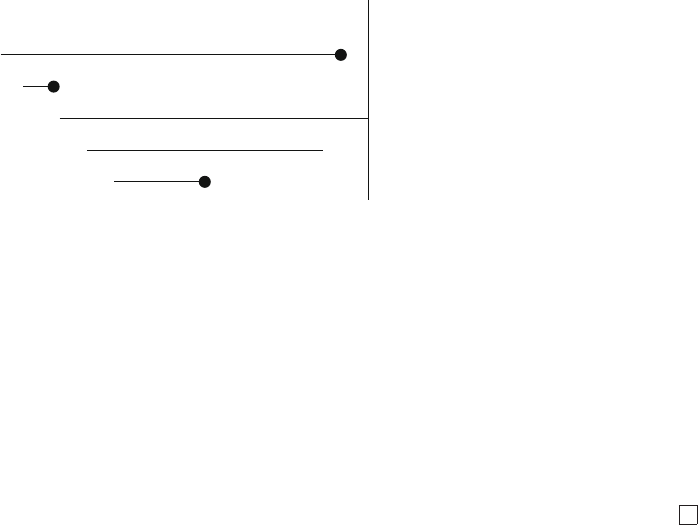
17.4 Homogeneous Failure Time Distributions 407

75 81

68+ 6868

5620 20 1

5252+

75 1

Termination of Study

Fig. 17.4 Some censored data. Circles denote events.

= −[u exp(−u)+exp(−u)]|

Λ(z )

=1− S(z)[Λ(z)+1].

Adding Λ(z)S(z)resultsin

E[Λ(min(T, z))] = 1 − S(z)=F (z). (17.18)

It follows that



i=1

Λ(min(T

,z)) estimates the expected number of failures

o ccurring before time z among the n subjects. 5

17.4 Homogeneous Failure Time Distributions

In this section we assume that each subject in the sample has the same dis-

tribution of the random variable T that represents the time until the event.

In particular, there are no covariables that describe diﬀerences between sub-

jects in the distribution of T .AsbeforeweuseS(t), λ(t), and Λ(t) to denote,

respectively, the survival, hazard, and cumulative hazar d functions.

The form of the true population survival distribution function S(t)isal-

most always unknown, and many distributional forms have been used for

describing failure time data. We consider ﬁrst the two most popular para-

metric sur vival distributions: the exponential and Weibull distributions. The

exponential distribution is a very simple one in which the hazard function is

constant; that is, λ(t)=λ . The cumulative hazard and survival functions

are then

Λ(t)=λt and

S(t)=exp(−Λ(t)) = exp(−λt). (17.19)

The median life length is Λ

−1

(log 2) or

408 17 Intro duction to Survival Analysis

0.5

= log(2)/λ. (17.20)

The time by which 1/2 of the subjects will have failed is then proportional to

the reciprocal of the constant hazard rate λ . This is true also of the expected

or mean life length, which is 1/λ.

The exponential distribution is o ne of the few distributions for which a

closed-form solution exists for the estimator of its parameter when censoring

is present. This estimator is a function of the number of events and the total

person-years of exposure. Methods based on person-years in fact implicitly

assume an exponential distribution. The exponential distribution is often used

to model events that occur “at random in time.”

323

It has the property that

the future lifetime of a subject is the same, no matter how “old” it is, or

Prob{T>t

+ t|T>t

} =Prob{T>t}. (17.21)

This “ageless” property also makes the exponential distribution a po or choice

for modeling human survival except over short time perio ds.

The Weibull distribution is a g eneralization of the exponential distribution.

Its hazard, cumulative hazard, and survival functions are given by

λ(t)=αγt

γ−1

Λ(t)=αt

(17.22)

S(t)=exp(−αt

The Weibull distribution with γ = 1 is an exponential distribution (with

constant hazard). When γ>1, its hazard is increasing with t,andwhen

γ<1 its hazard is decreasing. Figur e

17.5 depicts some of the shapes of

the hazard function that are possible. If T has a Weibull distribution, the

median of T is

0.5

= [(log 2)/α]

1/γ

. (17.23)

There are many other traditional parametric survival distributions, some of

which have hazards that are “bathtub shaped” as in Figure

17.3.

243, 323

The

restricted cubic spline function described in Section

2.4.5 is an alternative

basis for λ(t).

286, 287

This function family allows for any shape of smooth

λ(t) since the number of knots can be increased as needed, subject to the

number of events in the sample. Nonlinear terms in the spline function can

be tested to assess linearity of hazard (Rayleigh-ness) or constant hazard

(exponentiality).

The restricted cubic spline hazar d model with k knots is

(t)=a + bt +

k−2



j=1

(t), (17.24)

17.5 Nonparametric Estimation of S and Λ 409

0.0 0.2 0.4 0.6 0.8 1.0 1.2

Fig. 17.5 Some Weibull hazard functions with α = 1 and various values of γ.

where the w

(t) are the restricted cubic spline terms of Equation

2.25.There

terms are cubic terms in t. A set of knots v

,...,v

is selected from the

quantiles of the uncensore d failur e times (see Section

2.4.5 and [286]).

The cumulative hazard function for this model is

Λ(t)=at +

× quartic terms in t. (17.25)

Standard maximum likelihood theory is used to obtain estimates of the k

unknown parameters to derive, for example, smooth estimates of λ(t) with

conﬁdence bands. The ﬂexible estimates of S(t) using this method are as

eﬃcient as Kaplan–Meier estimates, but they are smooth and can be used as a

basis for modeling predictor variables. The spline hazard model is particularly

useful for ﬁtting steeply falling and gently rising hazard functions that are

characteristic of high-risk medical procedures.

17.5 Nonparametric Estimation of S and Λ

17.5.1 Kaplan–Meier Estimator

As the true form of the survival distribution is seldom known, it is useful to

estimate the distribution without making any assumptions. For many anal-

yses, this may be the last step, while in others this step helps one select a

statistical model for more in-depth analyses. When no event times are cen-

sored, a nonparametric estimator of S(t)is1−F

(t)whereF

(t) is the usual

410 17 Intro duction to Survival Analysis

Table 17.1 Kaplan-Meier computations

Day No. Subjects Deaths Censored Cumulative

At Risk Survival

12 100 1 0 99/100 = .99

30 99 2 1 97/99 × 99/100 = .97

60 96 0 3 96/96 × .97 = .97

72 93 3 0 90/93 × .97 = .94

.. .. .

empirical cumulative distribution function based on the observed failure times

,...,T

.LetS

(t) denote this empirical survival function. S

(t)isgiven

by the fraction of observed failure times that exceed t:

(t) = [number of T

>t]/n. (17.26)

When censoring is present, S(t) can be estimated (at least for t up until

the end of follow-up) by the Kaplan–Meier

333

product-limit estimato r. This

method is based on conditional probabilities. For example, suppose that ev-

ery subject has been followed for 39 days or has died within 39 days so that

the proportion of subjects surviving at least 39 days can be computed. After

39 days, some subjects may be lost to fo llow-up besides those removed from

follow-up because of death within 39 days. The proportion of those still fol-

lowed 39 days who survive day 40 is computed. The probability of surviving

40 days from study entry equals the probability of surviving day 40 after

living 39 days, multiplied by the chance of surviving 39 days.

The life table in Table

17.1 demonstrates the method in more detail. We

suppose that 100 subjects enter the study and none die or are lost before

day 12.

Times in a life table should b e measured as precisely as possible. If the

event being analyzed is death, the failure time should usually be speciﬁed

to the nearest day. We assume that deaths occur on the day indicated and

that being censored on a certain day implies the subject survived through the

end of that day. The data used in computing Kaplan–Meier estimates consist

of (Y

),i =1, 2,...,n using notation deﬁned previously. Primary data

collected to derive (Y

) usually consist of entry date, event date (if subject

failed), and censoring date (if subject did not fail). Instead, the entry da te,

date of event/censoring, and event/censoring indicator e

may be sp eciﬁed.

The Kaplan–Meier estimator is called the product-limit estimator because

it is the limiting case of actuarial survival estimates as the time periods

shrink so that an entry is made for each failure time. An entry need not

be in the table for censoring times (when no failures occur at that time) as

long as the number of subjects censored is subtracted from the next number

17.5 Nonparametric Estimation of S and Λ 411

Table 17.2 Summaries used in Kaplan-Meier computations

− d

)/n

1 1 7 1 6/7

2 3 6 2 4/6

3 9 2 1 1/2

at risk. Kaplan–Meier estimates are preferred to actuarial estimates because

they provide more resolution and make fewer assumptions. In constructing

a yearly actuarial life table, for example, it is traditionally assumed that

subjects censored between two years were followed 0.5 years.

The product-limit estimator is a nonparametric maximum likelihood es-

timator [

331, pp. 10–13]. The formula for the Kaplan–Meier product-limit

estimator of S(t) is as follows. Let k denote the number of failures in the

sample and let t

,...,t

denote the unique event times (ordered for ease

of calculation). Let d

denote the number of failures at t

and n

be the num-

ber of subjects at risk at time t

;thatis,n

= number o f failure/censoring

times ≥ t

. The estimator is then

(t)=



i:t

≤t

(1 − d

). (17.27)

The Kaplan–Meier estimator of Λ(t)isΛ

(t)=−log S

(t). An estimate

of quantile q of failure time is S

−1

(1 −q), if follow-up is long enough so that

(t)dropsaslowas1−q. If the last subject followed failed so that S

(t)

drops to zero, the expected failure time can be estimated by computing the

area under the Kaplan–Meier curve.

To demonstrate computation of S

(t), imagine a sample of failure times

given by

1336

910

where + denotes a censored time. The quantities needed to compute S

are

in Table

17.2.Thus

(t)=1, 0 ≤ t<1

=6/7=.85, 1 ≤ t<3

=(6/7)(4/6) = .57, 3 ≤ t<9 (17.28)

=(6/7)(4/6)(1/2) = .29, 9 ≤ t<10.

Note that the estimate of S(t) is undeﬁned for t>10 since not all subjects

have failed by t = 10 but no follow-up extends beyond t = 10. A graph of the

Kaplan–Meier estimate is found in Figure

17.6.

412 17 Intro duction to Survival Analysis

require(rms)

tt ← c(1,3,3,6,8,9,10)

stat ← c(1,1,1,0,0,1,0)

S ← Surv(tt, stat)

survplot(npsurv (S ∼ 1), conf="bands", n.risk =TRUE ,

xlab=expression (t))

survplot(npsurv (S ∼ 1, type="fleming-harrington ",

conf.int=FALSE ), add=TRUE , lty=3)

Survival Probability

012345678910

0.0

0.2

0.4

0.6

0.8

1.0

444

Fig. 17.6 Kaplan–Meier pro duct–limit estimator with 0.95 conﬁdence bands. The

Altschuler–Nelson–Aalen–Fleming–Harrington estimator is depicted with the dotted

lines.

The variance of S

(t) can be estimated using Greenwoo d’s formula [

331,

p. 14], a nd using normality of S

(t) in large samples this variance can

be used to derive a conﬁdence interval for S(t). A better method is to de-

rive an asymmetric conﬁdence interval for S(t) based on a symmetric in-

terval for log Λ(t). This latter method ensures that a conﬁdence limit does

not exceed one or fall below zero, and is more accurate since log Λ

(t)is

more normally distributed than S

(t). Once a conﬁdence interval, say [a, b]

is determined for log Λ(t), the conﬁdence interval for S(t) is computed by

[exp{−exp(b)}, exp{−exp(a)}]. The formula for an estimate of the variance

of interest is [

331, p. 15]:

Var{log Λ

(t)} =



i:t

≤t

/[n

− d

)]

{



i:t

≤t

log[(n

− d

)/n

]}

. (17.29)

17.6 Analysis of Multiple Endp oints 413

Letting s denote the square root of this variance estimate, an appr oximate

1 − α co nﬁdence interval for log Λ(t) is given by log Λ

(t) ±zs ,wherez is

the 1−α/2 standard normal critical value. After simpliﬁcation, the conﬁdence

interval for S(t) becomes

(t)

exp(±zs)

. (17.30)

Even though the log Λ basis for conﬁdence limits has theoretical advan-

tages, on the log −log scale the estimate of S(t) has the greatest instability

where much information is available: when S(t) falls just below 1.0. For that

reason, the recommended default conﬁdence limits are on the Λ(t) scale using

Var{Λ

(t)} =



i:t

≤t

− d

)]

. (17.31)

Letting s denote its square root, an approximate 1 −α conﬁdence interval for

S(t)isgivenby

exp(±zs)S

(t), (17.32)

truncated to [0, 1]. 7

17.5.2 Altschuler–Nelson Estimator

Altschuler

,Nelson

472

,Aalen

and Fleming and Harrington

196

proposed es-

timators of Λ(t)orofS(t) based on an estimator of Λ(t):

Λ(t)=



i:t

≤t

(t)=exp(−

Λ(t)). (17.33)

(t) has advantages over S

(t). First,



i=1

Λ(Y



i=1

[

605, Appendix 3]. In other words, the estimator gives the correct expected

number of events. Second, there is a wealth of asymptotic theory based on

the Altschuler–Nelson estimator.

196

See Figure 17.6 for an example of the S

(t) estimator. This estimator has

the same variance as S

(t) for large enough samples. 8

17.6 Analysis of Multiple Endpoints

Clinical studies frequently assess multiple endpoints. A cancer clinical trial

may, for example, involve recurrence of disease and death, whereas a car-

diovascular trial may involve nonfatal myo cardial infarction and death. End-

points may be combined, and the new event (e.g., time until infarction or

414 17 Intro duction to Survival Analysis

death) may be analyzed with any of the tools of sur vival analysis because only

the usual censoring mechanism is used. Sometimes the various endpoints may

need separate study, however, because they may have diﬀerent risk factors.

When the multiple endpoints represent multiple causes of a terminating

event (e.g., death), Prentice et al. have developed standard methods for an-

alyzing cause-speciﬁc hazards

513

[331, pp. 163–178]. Their methods allow

each cause of failure to be analyzed separately, censoring on the other causes.

They do not assume any mechanism for cause removal nor make any assump-

tions regarding the interrelation among causes of failure. However, analyses

of competing events using data where some causes of failure are removed in

a diﬀerent way from the original dataset will give rise to diﬀerent inferences.

When the multiple endpoints represent a mixture of fatal and nonfatal

outcomes, the analysis may be more complex. The same is true when one

wishes to jointly study an event-time endpoint and a repeated measurement.

17.6.1 Competing Risks

When events are independent, each event may also be analyzed separately by

censoring on all other events as well as censoring on loss to follow-up. This will

yield an unbiased estimate of an easily interpreted cause-speciﬁc λ(t)orS(t)

because censoring is no n-informative [

331, pp. 168–169]. One minus S

(t)

computed in this ma nner will correctly estimate the probability of failing from

the event in the absence of other events. Even when the competing events are

not independent, the cause-speciﬁc hazard model may lead to valid results,

but the resulting model does not allow one to estimate risks conditional on

removal of one or more causes of the event. See Kay

340

for a nice example

of compe ting r isks analysis when a treatment reduces the risk of death from

one cause but incr eases the risk of death from another cause.10

Larson and Dinse

376

have an interesting approach that jointly models the

time until (any) failure and the failure type. For r failure types, they use

an r-category polytomous logistic model to predict the probability of failing

from each cause. They assume that censoring is unrelated to cause of event.

17.6.2 Competing Dependent Risks

In many medical and epidemiologic studies one is interested in analyzing

multiple causes of death. If the goal is to estimate cause-speciﬁc failure prob-

abilities, treating subjects dying from extraneous causes as censored and

then computing the ordinary Kaplan–Meier estimate results in biased (high)

survival estimates

212, 225

.Ifcausem is of interest, the cause-speciﬁc hazard

17.6 Analysis of Multiple Endp oints 415

function is deﬁned as

(t) = lim

u→0

Pr{fail from cause m in [t, t + u)|alive at t}

. (17.34)

The cumulative incidence function or probability of failure from cause m by

time t is given by

(t)=



(u)S(u)du, (17.35)

where S(u) is the probability of surviving (ignoring cause of death), which

equals exp[−



(



(x))dx] [

212];[444, Chapter 10]; [102,408].Aspreviously

mentioned, 1−F

(t)=exp[−



(u)du] only if failures due to other causes

are eliminated and if the cause-speciﬁc hazard of interest remains unchanged

in doing so.

212

Again letting t

,...,t

denote the unique ordered failur e times, a non-

parametric estimate of F

(t)isgivenby

(t)=



i:t

≤t

i−1

), (17.36)

where d

is the number of failures of type m at time t

and n

is the number

of subjects at risk of failure at t

Pepe and others

494, 496, 497

showed how to use a combination of Kaplan–

Meier estimators to derive an estimator of the pr obability of being free of

event 1 by time t given event 2 has not occurred by time t (see also [

349]).

Let T

and T

denote, respectively, the times until events 1 and 2. Let S

(t)

and S

(t) denote, respectively, the two survival functions. Let us suppose

that event 1 is not a terminating event (e.g ., is no t death) and that even

after event 1 subjects are followed to a scertain occurrences of event 2. The

probability that T

>tgiven T

>tis

Prob{T

>t|T

>t} =

Prob{T

>tand T

>t}

Prob{T

>t}

(t)

, (17.37)

where S

(t) is the survival function for min(T

), the earlier of the two

events. Since S

(t) does not involve any informative censoring (assuming as

always that loss to follow-up is non-informative), S

may be estimated by

the Kaplan–Meier estimator S

(or by S

). For the type of event 1 we

have discussed above, S

can also be estimated without bia s by S

.Thus

we estimate, for example, the probability that a subject still alive at time t

will be free of myocardial infarction as of time t by S

416 17 Intro duction to Survival Analysis

Another quantity that can easily be computed from ordinary survival es-

timates is S

(t) − S

(t)=[1−S

(t)] − [1 − S

(t)], which is the probability

that event 1 occurs by time t and that event 2 has not occurred by time t.

The ratio estimate above is used to estimate the survival function for one

event given that another has not occurred. Another function of interest is

the crude survival function which is a marginal distribution; that is, it is the

probability that T

>twhether or not event 2 occurs:

362

(t)=1− F

(t)

(t)=Prob{T

≤ t}, (17.38)

where F

(t)isthecrude incidence function deﬁned previously. Note that the

≤ t implies that the occurrence of event 1 is part of the probability being

computed. If event 2 is a terminating event so that some subjects can never

suﬀer event 1, the crude survival function for T

will never drop to zero. The

crude survival function can be interpreted as the survival distribution of W

where W = T

if T

and W = ∞ otherwise.

362

17.6.3 State Transitions and Multiple Types

of Nonfatal Events

In many studies there is one ﬁnal, absorbing state (death, all causes) and mul-

tiple live states. The live states may represent diﬀerent health states or phases

of a disease. For example, subjects may be completely free of cancer, have an

isolated tumor, metastasize to a distant organ, and die. Unlike this example,

the live states need not have a deﬁnite or dering. One may be interested in es-

timating tr ansition probabilities, for example, the probability π

)that

an individual in state i at time t

is in state j after an additional time t

Strauss and Shavelle

596

have developed an extended Kaplan–Meier estimator

for this situation. Let S

(t|t

) denote the ordinary Kaplan–Meier estimate

of the probability of not dying before time t (ignoring distinctions between

multiple live states) for a cohort of subjects beginning follow-up at time t

in state i. This is an estimate of the probability of surviving an additional t

time units (in any live state) given that the subject was alive and in state i

at time t

. Strauss and Shavelle’s estimator is given by

)

), (17.39)

where n

) is the number of subjects in live state i at time t

who are

alive and uncensored t

time units later, and n

)isthenumberofsuch

subjects in state jt

time units beyond t

.12

17.6 Analysis of Multiple Endp oints 417

17.6.4 Joint Analysis of Time and Severity

of an Event

In some studies, an endpoint is given more weight if it occurs earlier or

if it is more severe clinically, or both. For example, the event of interest

may be myocardial infarction, which may be of any severity from minimal

damage to the left ventricle to a fatal infarction. Berridge and Whitehead

have pr ovided a pro mising model for the analysis of such endpoints. Their

method assumes that the severity of endpoints which do occur is measured

on an ordinal categorical scale and that severity is assessed at the time of

the event. Berridge and Whitehead’s example was time until ﬁrst headache,

with severity of headaches graded on an ordinal scale. They prop osed a joint

hazard of an individual who responds with ordered category j:

(t)=λ(t)π

(t), (17.40)

where λ(t) is the hazard for the failure time and π

(t) is the proba bility of an

individual having event severity j given she fails at time t. Note that a shift

in the distribution of response severity is allowed as the time until the event

increases. 13

17.6.5 Analysis of Multiple Events

It is common to choose as an endpoint in a clinical trial an event that can

recur. Examples include myocardial infarction, gastric ulcer, pregnancy, and

infection. Using only the time until the ﬁrst event can result in a loss of

statistical information and power.

There are specialized multivariate survival

models (whose assumptions are extremely diﬃcult to verify) for handling this

setup, but in many cases a simpler approach will be eﬃcient.

The simpler approach involves modeling the marg inal distribution of the

time until each event.

407, 495

Here one forms one record per subject per event,

and the survival time is the time to the ﬁrst event for the ﬁrst record, or is

the time from the previous event to the next event for all later records. This

approach yields consistent estimates of distribution parameters as long as the

marginal distributions are correctly speciﬁed.

655

One can allow the number of

previous events to inﬂuence the hazard functio n of another event by modeling

this count as a covariable.

The multiple events within subject are not indep endent, so variance esti-

mates must be corr ected for intracluster correlation. The clustered sandwich

covariance matrix estimator describ ed in Section

9.5 and in

[

407] will provide

An exception to this is the case in which once an event occurs for the ﬁrst time, that

event is likely to recur multiple times for any patient. Then the latter occurrences are

redundant.

418 17 Intro duction to Survival Analysis

consistent estimates of variances and covariances even if the events are de-

pendent. Lin

407

also discussed how this method can easily be used to model

multiple events of diﬀering types.14

17.7 R Functions

The event.chart function of Lee et al.

394

will draw a variety of charts for dis-

playing raw survival time data, for both single a nd multiple events per sub-

ject. Relationships with covariables can also be displayed. The event.history

function of Dubin et al.

166

draws an event history graph for right-censored

survival da ta, including time-dependent covariate status. These function are

in the Hmisc package.

The analyses described in this chapter can b e viewed as special cases of the

Cox proportional hazards model.

132

The programs for Cox model analyses

describedinSection20.13 can be used to obtain the results described here, as

long as there is at least one stratiﬁcation factor in the model. There are, how-

ever, several R functions that are pertinent to the homog eneous or stratiﬁed

case. The R function survfit, and its particular renditions of the print, plot,

lines, and points generic functions (all part of the survival package written

by Terry Therneau), will compute, print, and plot Kaplan–Meier and Nelson

survival estimates. Conﬁdence intervals for S(t)maybebasedonS, Λ,or

log Λ.Therms package’s front-end to the survival package’s survfit function

is npsurv for “nonparametric survival”. It and other functions described in

later chapters use Therneau’s Surv function to combine the response variable

and event indicator into a single R “survival time” object. In its simplest form,

use Surv(y, event),wherey is the failure/right–censoring time and event is

the event/censoring indicator, usually coded T/F,0=censored1=eventor

1 = censored 2 = event. If the event status variable has other coding (e.g., 3

means death), use Surv(y, s==3). To handle interval time-dependent covari-

ables, or to use Andersen and Gill’s counting process formulation of the Cox

model,

use the notation Surv(tstart, tstop, status). The counting process

notation allows subjects to enter and leave risk sets at random. For each

time interval for each subject, the interval is made up of tstart<t≤tstop.

For time-dependent stratiﬁcation, there is an optio nal origin argument to

Surv that indicates the hazard shape time origin at the time o f crossover

to a new stratum. A type ar gument is used to handle left– and interval–

censoring, especially for parametric survival models. Possible values of type

are "right","left","interval","counting","interval2","mstate".

The Surv expression will usually be used inside ano ther function, but it is

ﬁne to save the result of Surv in another object and to use this object in the

particular ﬁtting function.

npsurv is invoked by the following, with default parameter settings indi-

cated.

17.7 R Functions 419

require(rms)

units(y) ← "Month "

# Default is "Day" - used for axis labels , etc.

npsurv (Surv(y, event) ∼ svar1 + svar2 + ... , data , subset ,

type=c("kaplan-meier", "fleming-harrington ", "fh2"),

error=c("greenwood", "tsiatis"), se.fit =TRUE ,

conf.int=.95,

conf.type=c("log","log-log","plain ","none"), ...)

If there are no stratiﬁcation variables (svar1,...),omitthem.Toprintatable

of estimates, use

f ← npsurv (...)

print(f) # print brief summary of f

summary(f, times , censored=FALSE ) # in survival

For failure times stored in days, use

f ← npsurv (Surv(futime , event) ∼ sex)

summary(f, seq(30, 180, by=30))

to print monthly estimates.

There is a plot method To plot the object returned by survfit and npsurv.

This invokes plot.survfit.

Objects created by npsurv can be passed to the more comprehensive plot-

ting function survplot (here, actually survplot.npsurv) for other options that

include automatic curve labeling and showing the number of subjects at risk

at selected times. See Figure

17.6 for an example. Stratiﬁed estimates, with

four treatments distinguished by line type and curve labels, could be drawn

units(y) ← "Year"

f ← npsurv (Surv(y, stat) ∼ treatment)

survplot(f, ylab="Fraction Pain-Free")

The groupkm in rms computes and optionally plots S

(u)orlogΛ

(u)(if

loglog=TRUE)forﬁxedu with automatic stratiﬁcatio n on a continuous predic-

tor x.Asincut2 (Section

6.2) you can specify the number of subjects per

interval (default is m=50), the number of quantile groups (g), or the actual cut-

points (cuts). groupkm plots the survival or log–log survival estimate against

mean x in each x interval.

The bootkm function in the Hmisc package bootstraps Kaplan–Meier sur-

vival estimates or Kaplan–Meier estimates of quantiles of the survival time

distribution. It is easy to use bootkm to compute, for example, a nonparametric

conﬁdence interval for the ratio of median survival times for two groups.

See the Web site for a list of functions from other users for nonparametric

estimation of S(t) with left–, right–, and interval–censored data. The adaptive

linear spline log-hazard ﬁtting function heft

361

is freely available.

420 17 Intro duction to Survival Analysis

17.8 Further Reading

1 Some excellent general references for survival analysis are [57, 83, 114, 133, 154,

197, 282, 308, 331, 350, 382, 392, 444, 484, 574, 604]. Govindarajulu et al.

229

have

a n ice review of frailty models in survival analysis, for handling clustered time-

to-event data.

See Goldman,

220

Bull and Spiegelhalter,

, Lee et al.

394

, and Dubin et al.

166

for ways to construct descriptive graphs depicting right–censored data.

Some useful references for left–truncation are [83,112,244,524]. Mandel

435

care-

fully described the diﬀerence b etween censoring and truncation.

See [384, p. 164] for some ideas for detecting informative censoring. Bilker and

Wang

discuss right–truncation and contrast it with right–censoring.

Arjas

has applications based on properties of the cumulative hazard function.

Kooperberg et al.

361, 594

have an adaptive method for ﬁtting hazard functions

using linear splines in the log hazard. Binquet et al.

studied a related approach

using quadratic splines. Mudholkar et al.

466

presented a generalized Weibull

model allowing for a variety of hazard shapes.

Hollander et al.

299

provide a nonparametric simultaneous conﬁdence band for

S(t), surprisingly using likelihoo d ratio methods. Miller

459

showed that if the

parametric form of S(t) is known to be Weibull with known shape parameter (an

unlikely scenario), the Kaplan–Meier estimator is very ineﬃcient (i.e., has high

variance) when compared with the parametric maximum likelihood estimator.

See [

666] for a discussion of how the eﬃciency of Kaplan–Meier estimators can

be improved by interpolation as opposed to piecewise ﬂat step functions. That

paper also discusses a va riety of other estimators, some of which are signiﬁcantly

more eﬃcient than Kaplan–Meier.

See [112,244,438,570,614,619] for methods of estimating S or Λ in the presence

of left–truncation. See Turnbull

616

for nonparametric estimation of S(t)with

left–, right–, and interval–censoring, and Kooperberg and Clarkson

360

for a

ﬂexible parametric approach to modeling that allows for interval–censoring.

Lindsey and Ryan

413

have a nice tutorial on the analysis of interval–censored

data.

Hogan and Laird

297, 298

develop ed methods for dealing with mixtures of fa-

tal and nonfatal outcomes, including some ideas for handling outcome-related

dropouts on the repeated measurements. See also Finkelstein and Schoenfeld.

193

The 30 April 1997 issue of Statistics in Medicine (Vol. 16) is devoted to methods

for analyzing multiple endpoints as well as designing multiple endpoint stud-

ies. The papers in that issue are invaluable, as is Therneau and Hamilton

606

and Therneau and Grambsch.

604

Huang and Wang

311

presented a joint model

for recurrent events and a terminating even t, addressing such issues as the fre-

quency of recurren t ev ents by the time of the terminating event.

See Lunn and McNeil

429

and Marubini and Valsecchi [444, Chapter 10] for

practical approaches to analyzing competing risks using ordinary Cox propor-

tional hazards models. A nice overview of competing risks with comparisons of

various approaches is found in Tai et al.

599

,Geskus

214

, and Koller et al.

358

Bryant and Dignam

developed a semiparametric procedure in which com-

peting risks are adjusted for nonparametrically while a parametric cumulative

incidence function is used for the event of interest, to gain precision. Fine and

Gray

192

developed methods for analyzing competing risks by estimating sub-

distribution functions. Nishikawa et al.

478

developed some novel approaches to

competing risk analysis involving time to adverse drug even ts competing with

time to withdrawal from therapy. They also dealt with diﬀerent severities of

events in an interesting way. Putter et al.

517

has a nice tutorial on competing

risks, multi-state mo dels, and associated R software. Fiocco et al.

194

developed

17.9 Problems 421

an approac h to avoid the problems caused by having to estimate a large num-

ber of regression coeﬃcients in multi-state models. Ambrogi et al.

provide

clinically useful estimates from competing risks analyses.

Jiang, Chappell, and Fine

322

present methods for estimating the distribution

of event times of nonfatal events in the presence of terminating events suc h as

death.

Shen and Thall

568

have developed a ﬂexible parametric approach to multi-state

survival analysis.

Lancar et al.

372

developed a method for analyzing repeated events of varying

severities.

Lawless and Nadeau

384

have a very good description of models dealing with

recurrent events. They use the notion of the cumulative mean function,which

is the expected number of events experienced by a subject by a certain time.

Lawless

383

contrasts this approach with other approaches. See Aalen et al.

for a nice example in which multivariate failure times (time to failure of ﬁll-

ings in multiple teeth per subject) are analyzed. Francis and Fuller

204

devel-

oped a graphical device for depicting complex event history data. Therneau and

Hamilton

606

have very informative comparisons of various methods for model-

ing multiple events, showing the importance of whether the analyst starts the

clock over after each event. Kelly and Lim

343

have another very useful paper

comparing various methods for analyzing recurrent events. Wang and Chang

650

demonstrated the diﬃculty of using Kaplan–Meier estimates for recurrence time

data.

17.9 Problems

1. Make a rough drawing of a hazard function from birth for a man who de-

velops signiﬁcant coronary a rtery disease at age 50 and under goes coronary

artery bypass surgery at age 55.

2. Deﬁne in words the relationship between the hazard function and the sur-

vival function.

3. In a study of the life expectancy of light bulbs as a function of the bulb’s

wattage, 100 bulbs of various wattage ratings were tested until each had

failed. What is wrong with using the product-moment linear correlation

test to test whether wattage is associated with life length concerning (a)

distributional assumptions and (b) other assumptions?

4. A placebo-controlled study is undertaken to ascertain whether a new drug

decreases mortality. During the study, some subjects are withdrawn be-

cause of moderate to severe side eﬀects. Assessment o f side eﬀects and

withdrawal o f patients is done on a blinded basis. What statistical tech-

nique can be used to obtain an unbiased treatment comparison of survival

times? State at least one eﬃcacy endpoint that can be analyzed unbiasedly.

5. Consider long -term follow-up of patients in the

support dataset. What pro-

portion of the patients have censored survival times? Does this imply that

one cannot make accurate estimates of chances of survival? Make a his-

togram or empirical distribution function estimate of the censored follow-

up times. Wha t is the typical follow-up duration for a patient in the study

422 17 Intro duction to Survival Analysis

who has survived so far? What is the typical survival time for patients who

have died? Taking censoring into account, what is the median survival time

from the Kaplan–Meier estimate of the overall survival function? Estimate

the median graphically or using any other sensible method.

6. Plot Kaplan–Meier survival function estimates stratiﬁed by dzclass.Esti-

mate the median survival time and the ﬁrst quartile of time until death

for each of the four disease classes.

7. Rep eat Problem

6 except for tertiles of meanbp.

8. The commonly used log-rank test for comparing survival times between

groups of patients is a special case of the test of association between the

grouping variable and survival time in a Cox proportional hazards regres-

sion model. Depending on how one handles tied failure times, the log-rank

statistic exactly equals the scor e χ

statistic from the Cox model, and

the likelihood ratio and Wald χ

test statistics are also appropriate. To

obtain global score or LR χ

tests and P -values you can use a statement as

the following, where cph is in the rms package. It is similar to the survival

package’s coxph function.

cph(Survobject ∼ predictor)

Here Survobject is a survival time object created by the Surv function. Ob-

tain the log-rank (score) χ

statistic, degrees of freedom, and P -value for

testing for diﬀerences in survival time between levels of dzclass. Interpret

this test, referring to the graph you produced in Problem

6 if needed.

9. Do preliminary analyses of survival time using the Mayo Clinic primary bil-

iary cirrhosis dataset described in Section

8.9. Make graphs of Altschuler–

Nelson or Kaplan–Meier surviva l estimates stratiﬁed separately by a few

categorical predictors and by categorized versions of one or two continuous

predictors. Estimate median failure time for the various strata. You may

want to suppress conﬁdence bands when showing multiple strata on one

graph. See

[

361] for parametric ﬁts to the survival and hazard function for

this dataset.

Chapter 18

Parametric Survival Models

18.1 Homogeneous Models (No Predictors)

The nonparametric estimator of S(t) is a very good descriptive statistic for

displaying sur vival data . For many purposes, however, one may want to make

more assumptions to allow the data to be modeled in more detail. By speci-

fying a functional form for S(t) and estimating any unknown parameters in

this function, one can

1. easily compute selected quantiles of the survival distribution;

2. estimate (usually by extrapolation) the exp ected failure time;

3. derive a concise equation and smooth function for estimating S(t), Λ(t),

and λ(t); and

4. estimate S(t) more precisely than S

(t)orS

(t) if the parametric form

is correctly speciﬁed.

18.1.1 Speciﬁc Models

Parametric modeling requires choosing one or more distributions. The Weibull

and e xponential distributions were discussed in Chapter

18. Other commonly

used survival distributions are obtained by transforming T andusingastan-

dard distribution. The log transformation is most commonly employed. The

log-normal distribution speciﬁes that log(T ) has a normal distribution with

mean μ and variance σ

. Stated another way, log(T ) ∼ μ + σǫ,whereǫ

has a standard normal distribution. Then S(t)=1− Φ((log(t) − μ)/σ),

where Φ is the standard normal cumulative distribution function. The log-

logistic distribution is given by S(t) = [1 + exp(−(log(t) − μ)/σ)]

−1

.Here

log(T ) ∼ μ+σǫ where ǫ follows a logistic distribution [1+exp(−u)]

−1

.Thelog

F.E. Harrell, Jr., Regression Modeling Strategies, Springer Series

in Statistics, DOI 10.1007/978-3-319-19425-7

423

424 18 Parametric Survival Models

extreme value distribution is given by S(t)=exp[−exp((log(t) −μ)/σ )], and

log(T ) ∼ μ + σǫ,whereǫ ∼ 1 − exp[−exp(u)].

The generalized gamma and generalized F distributions provide a richer

var i ety of distribution and hazard functions

127, 128

. Spline hazard

models

286, 287, 361

are other excellent alternatives.

18.1.2 Estimation

Maximum likelihood (ML) estimation is used to estimate the unknown

parameters of S(t). The general method presented in Chapter

9 must be

augmented, however, to allow for censored failure times. The basic idea is a s

follows. Again let T be a random variable representing time until the event,

be the (possibly censored) failure time for the ith observation, and Y

denote the obser ved failure or censoring time min(T

), where C

is the

censoring time. If Y

is uncensored, observation i contributes a factor to the

likelihood equal to the density functio n fo r T evaluated at Y

, f (Y

). If Y

instead represents a censored time so that T

= Y

, it is only known that

exceeds Y

. The contribution to the likelihood function is the probability

that T

(equal to Prob{T

}). This probability is S(Y

). The joint

likelihood over all observations i =1, 2,...,n is

L =



i:Y

uncensored

f(Y

)



i:Y

censored

S(Y

). (18.1)

There is one more component to L: the distribution of censoring times if

these are not ﬁxed in advance. Recall that we assume that censoring is non-

informative, that is, it is independent of the risk of the event. This inde-

pe ndence implies that the likelihood component of the censoring distribution

simply multiplies L and that the censoring distribution contains little infor-

mation about the survival distribution. In addition, the censoring distribution

may be very diﬃcult to specify. For these r easons we can maximize L sepa-

rately to estimate parameters of S(t) and ignore the censoring distribution.

Recalling that f (t)=λ(t)S(t)andΛ(t)=−log S(t), the log likelihood

canbewrittenas

log L =



i:Y

uncensored

log λ(Y

) −



i=1

Λ(Y

). (18.2)

All observations then contribute an amount to the log likelihood equal to the

negative of the cumulative hazard evaluated at the failure/censoring time.

In addition, uncensored observations contribute an amount equal to the log

of the hazard function evaluated at the time of failure. Once L or log L

is speciﬁed, the general ML methods outlined earlier can be used without

18.1 Homogeneous Models (No Predictors) 425

change in most situations. The principal diﬀerence is that censored observa-

tions contribute less information to the statistical inference than uncensored

observations. For distributions such as the log-normal that are written only

in terms of S(t), it may be easier to write the likelihood in terms of S(t)

and f (t).

As an example, we turn to the exponential distribution, for which log

L has a simple form that can be maximized explicitly. Recall that for this

distribution λ(t)=λ and Λ(t)=λt. Therefore,

log L =



i:Y

uncensored

log λ −



i=1

λY

. (18.3)

Letting n

denote the numb er of uncensored event times,

log L = n

log λ −



i=1

λY

. (18.4)

Letting w denote the sum of all failure/censoring times (“person years of

exposure”):

w =



i=1

, (18.5)

the derivatives of log L are given by

∂ log L

∂λ

= n

/λ − w

∂

log L

∂λ

= −n

/λ

. (18.6)

Equating the derivative of log L to zero implies that the MLE of λ is

λ = n

/w (18.7)

or the numb er of failures per person-years of exposure. By inserting the MLE

of λ into the formula for the second derivative we obtain the observed esti-

mated information, w

. The estimated variance of

λ is thus n

and

the standard error is n

1/2

/w. The precision of the estimate depends primarily

on n

Recall that the expected life length μ is 1/λ for the exponential distribu-

tion. The MLE of μ is w/n

and its estimated variance is w

.TheMLE

of S(t),

S(t), is exp(−

λt), and the estima ted variance of log(

Λ(t)) is simply

1/n

As an example, consider the sample listed previously,

1336

910

426 18 Parametric Survival Models

Here n

=4andw = 40, so the MLE of λ is 0.1 failure per person-period.

The estimated standard error is 2/40=0.05. Estimated expected life length

is 10 units with a standard error of 5 units. Estimated median failure time is

log(2)/0.1=6.931. The estimated survival function is exp(−0.1t), which at

t =1, 3, 9, 10 yields 0.90, 0.74, 0.41, and 0.37, which can be compared to the

product limit estimates listed earlier (0.85, 0.57, 0.29, 0.29).

Now consider the Weibull distribution. The log likelihood function is

log L =



i:Y

uncensored

log[αγY

γ−1

] −



i=1

αY

. (18.8)

Although log L can be simpliﬁed somewhat, it cannot be solved explicitly for

α and γ. An iterative method such as the Newton–Raphson method is used

to compute the MLEs of α and γ. Once these estimates are obtained, the

estimated variance–covariance matrix and other der ived quantities such as

S(t) can b e obtained in the usual manner.

For the dataset used in the exponential ﬁt, the Weibull ﬁt follows.

ˆα =0.0728

ˆγ =1.164

S(t)=exp(−0.0728t

1.164

) (18.9)

−1

(0.5) = [(log 2)/ˆα]

1/ˆγ

=6.935 (estimated median).

This ﬁt is very clo se to the exponential ﬁt since ˆγ is near 1.0. Note that the

two medians are almost equal. The predicted survival probabilities for the

Weibull model for t =1, 3, 9, 10 are, respectively, 0.93, 0.77, 0.39, 0.35.

Sometimes a formal test can b e made to assess the ﬁt of the prop osed

parametric survival distribution. For the data just analyzed, a formal test of

exponentiality versus a Weibull alternative is obtained by testing H

: γ =1

in the Weibull model. A score test yielded χ

=0.14 with 1 d.f., p =0.7,

showing little evidence for non-exponentiality (note that the sample size is

too small for this test to have any power).

18.1.3 Assessment of Model Fit

The ﬁt of the hypothesized survival distribution can often be checked eas-

ily using graphical methods. Nonparametric estimates of S(t)andΛ(t)

are primary tools for this purpose. For example, the Weibull distribution

S(t)=exp(−αt

) can be rewritten by taking logarithms twice:

log[−log S(t)] = log Λ(t) = log α + γ(log t). (18.10)

18.2 Parametric Proportional Hazards Models 427

The ﬁt of a Weibull model can be assessed by plotting log

Λ(t)versuslogt

and checking whether the curve is approximately linear . Also , the plotted

curve provides approximate estimates of α (the antilog of the intercept) and

γ (the slope). Since an exponential distribution is a special case of a Weibull

distribution when γ = 1, exponentially distributed data will tend to have a

graph that is linear with a slope of 1.

For any a ssumed distribution S(t), a graphical assessment of goodness of

ﬁtcanbemadebyplottingS

−1

(t)] or S

−1

(t)] against t and checking

for linearity. For log distributions, S speciﬁes the distribution of log(T ), so

we plot against log t . For a log-normal distribution we thus plot Φ

−1

(t)]

against log t,whereΦ

−1

is the inverse of the standard normal cumulative

distribution function. For a log-logistic distribution we plot logit[S

(t)] versus

log t. For an extreme value distribution we use log −log plots as with the

Weibull distribution. Parametric model ﬁts can also be checked by plotting

the ﬁtted

S(t)andS

(t) against t on the same graph.

18.2 Parametric Proportional Hazards Models

In this sectio n we present one way to generalize the survival model to a

survival regression mo del. In other words, we allow the sample to b e hetero-

geneous by adding predictor varia bles X = {X

,...,X

}.Aswithother

regression models, X can represent a mixture of binary, polytomous, continu-

ous, spline-expanded, and even ordinal predictors (if the categories are scored

to satisfy the linearity assumption). Before discussing ways in which the re-

gression pa rt of a survival model might be speciﬁed, ﬁrst r ecall how regression

eﬀects have been modeled in other settings. In multiple linear regression, the

regression eﬀect Xβ = β

+ β

+ ...+ β

can be thought of

as an increment in the expected value of the response Y . In binary logistic

regression, Xβ speciﬁes the log odds that Y =1,orexp(Xβ) multiplies the

odds that Y =1.

18.2.1 Model

The most widely used survival regression speciﬁcation is to allow the hazard

function λ(t) to be multiplied by exp(Xβ). The survival model is thus gener-

alized from a hazard function λ(t) for the failure time T to a hazard function

λ(t)exp(Xβ) for the failure time given the predictors X:

λ(t|X)=λ(t)exp(Xβ). (18.11)

428 18 Parametric Survival Models

This regression formulation is called the proportional hazar ds (PH) model.

The λ(t)partofλ(t|X) is sometimes called an underlying hazard function or

a hazard function for a standar d subject, which is a subject with Xβ =0.Any

parametric hazard function can b e used for λ(t), and as we show later, λ(t)

can be left completely unspeciﬁed without sacriﬁcing the ability to estimate

β, by the use of Cox’s semi-parametric PH model.

132

Depending on whether

the underlying hazard function λ(t) has a constant scale parameter, Xβ may

or may not include an intercept β

. The term exp(Xβ) can be called a relative

hazard function and in many cases it is the function of primary interest as it

describes the (relative) eﬀects of the predictors.

The PH model can also be written in terms of the cumulative hazard and

survival functions:

Λ(t|X)=Λ(t)exp(Xβ)

S(t|X)=exp[−Λ(t)exp(Xβ)] = exp[−Λ(t)]

exp(Xβ)

. (18.12)

Λ(t) is an “underlying” cumulative hazard function. S(t|X), the probability

of surviving past time t given the values of the predictors X, can also be

written as

S(t|X)=S(t)

exp(Xβ)

, (18.13)

where S(t) is the “underlying” survival distr ibution, exp(− Λ(t)). The eﬀect

of the predicto rs is to multiply the hazard and cumulative hazard functions

by a factor exp(Xβ), or equivalently to raise the survival function to a power

equal to exp(Xβ).

18.2.2 Model Assumptions and Interpretation

of Parameters

In the general regression notation of Section

2.2, the log hazard or log cumu-

lative hazard can be used as the prop erty of the response T evaluated at time

t that allows distributional and regression parts to be isolated and checked.

The PH model can be linearized with respect to Xβ using the following

identities.

log λ(t|X) = log λ(t)+Xβ

log Λ(t|X) = log Λ(t)+Xβ. (18.14)

No matter which of the three model statements are used, there are certain

assumptions in a parametric PH survival model. These assumptions are listed

below.

1. The true form of the underlying functions (λ, Λ,andS) sho uld be speciﬁed

correctly.

18.2 Parametric Proportional Hazards Models 429

2. The relationship between the predictors and log hazard or log cumulative

hazard should be linear in its simplest form. In the absence of interaction

terms, the predictors should also operate a dditively.

3. The way in which the predictors aﬀect the distribution o f the response

should be by multiplying the hazar d or cumulative hazard by exp(Xβ)

or equiva lently by adding Xβ to the log hazard or log cumulative hazard

at each t. The eﬀect of the predictors is assumed to be the same at all

values of t since log λ(t) can be separated from Xβ. In other words, the

PH assumption implies no t by predictor interaction.

The regression coeﬃcient for X

, β

, is the increase in log hazard or log

cumulative hazard at any ﬁxed po int in time if X

is increased by one unit

and all other predictors are held constant. This can be written formally as

=logλ(t|X

,...,X

+1,X

j+1

,...,X

) −log λ(t|X

,...,X

(18.15)

which is equivalent to the log of the ratio of the hazards at time t.The

regression coeﬃcient can just as easily be written in terms of a ratio of hazards

at time t. The ratio of hazards at X

+ d versus X

, all other factors held

constant, is exp(β

d). Thus the eﬀect of increasing X

by d is to increase the

hazard of the event by a factor of exp(β

d) at all points in time, assuming X

is linearly related to log λ(t). In general, the ratio of hazards for an individual

with predictor variable values X

∗

compared to an individual with predictors

X is

∗

: X hazard ratio = [λ(t)exp(X

∗

β)]/[λ(t)exp(Xβ)]

=exp(X

∗

β)/ exp(Xβ)=exp[(X

∗

− X)β]. (18.16)

If there is only one predictor X

and that predicto r is binary, the PH model

can be written

λ(t|X

=0)=λ(t)

λ(t|X

=1)=λ(t)exp(β

). (18.17)

Here exp(β

)istheX

=1:X

= 0 hazard ratio . This simple case has

no regression assumption but assumes PH and a form for λ(t). If the single

predictor X

is continuous, the model becomes

λ(t|X

)=λ(t)exp(β

X). (18.18)

Without further modiﬁcation (such as ta king a transformation of the predic-

tor), the model assumes a straight line in the log hazar d or that for all t,an

increase in X by one unit increases the hazard by a factor of exp(β

As in logistic regression, much more general regression speciﬁcations can

be made, including interaction eﬀects. Unlike logistic regression, however, a

model containing, say age, sex, and age × sex interaction is not equivalent to

430 18 Parametric Survival Models

ﬁtting two separate models. This is because even though males and females

are allowed to have unequal age slopes, both sexes are assumed to have the

Table 18.1 Mortality diﬀerences and ratios when hazard ratio is 0.5

Subject 5-Year Diﬀerence Mortality

Survival Ratio (T/C)

1 0.98 0.99 0.01 0.01/0.02 = 0.5

2 0.80 0.89 0.09 0.11/0.2 = 0.55

3 0.25 0.50 0.25 0.5/0.75 = 0.67

underlying hazard function proportional to λ(t) (i.e., the PH assumption

holds for sex in addition to age).

18.2.3 Hazard Ratio, Risk Ratio, and Risk

Diﬀerence

Other ways of modeling predictors can also be speciﬁed besides a multiplica-

tive eﬀect on the hazard. For example, one could postulate that the eﬀect of

a predictor is to add to the hazard of failure instead of to multiply it by a

factor. The eﬀect of a predictor could also be described in terms of a mor-

tality ratio (relative risk), risk diﬀerence, odds ratio, or increase in expected

failure time. However, just as an odds ratio is a natural way to describe an

eﬀect on a binary response, a hazard ratio is often a natural way to describe

an eﬀect on survival time. One reason is that a hazard ratio can be constant.

Table

18.1 provides treated (T) to co ntrol (C) survival (mortality) dif-

ferences and mortality ratios for three hypothetical types of subjects. We

suppose that subjects 1, 2, a nd 3 have increasingly worse prognostic factors.

For example, the age at baseline of the subjects might be 30, 50, and 70 years,

respectively. We assume that the treatment aﬀects the hazard by a constant

multiple of 0.5 (i.e., PH is in eﬀect and the constant hazard ratio is 0.5). Note

that S

= S

0.5

. Notice that the mortality diﬀerence and ratio depend on the

survival of the control subject. A control subject having “good” predictor

values will leave little room for an improved prognosis from the treatment.

The hazard ratio is a basis for describing the mechanism of an eﬀect. In the

above example, it is reasonable that the treatment aﬀect each subject by low-

ering her hazard of death by a factor of 2, even though less sick subjects have

a low mortality diﬀerence. Hazard ratios also lead to good statistical tests

for diﬀerences in survival patterns and to predictive models. Once the model

is developed, however, survival diﬀerences may better capture the impact of

a risk factor. Absolute surviva l diﬀerences rather than relative diﬀerences

18.2 Parametric Proportional Hazards Models 431

(hazard ratios) also relate more closely to statistical power. For example,

even if the eﬀect of a treatment is to halve the hazard rate, a population

where the control survival is 0.99 will require a much larger sample than will

a population where the control survival is 0.3.

Figure

18.1 depicts the relationship between survival S(t)ofacontrol

subject at any time t, relative reduction i n hazard (h), and diﬀerence in

survival S(t) −S(t)

. This ﬁgure demonstrates that absolute clinical beneﬁt

0.0 0.2 0.4 0.6 0.8 1.0

0.0

0.1

0.2

0.3

0.4

0.5

0.6

0.7

Survival for Control Subject

Improvement in Survival

0.1

0.2

0.3

0.4

0.5

0.6

0.7

0.8

0.9

Fig. 18.1 Absolute clinical beneﬁt as a function of survival in a control subject and

the relative beneﬁt (hazard ratio). The hazard ratios are given for each curve.

is primar ily a function of the baseline risk of a subject. Clinical beneﬁt will

also be a function of factors that interact with treatment, that is, factors

that modify the relative beneﬁt of treatment. Once a model is developed

for estimating S(t|X), this model can be used to estimate absolute beneﬁt

as a function of baseline risk factors as well as factors that interact with a

treatment. Let X

be a binary treatment indicator and let A = {X

,...,X

}

be the other factors (which for convenience we assume do not interact with

). Then the estimate of S(t|X

=0,A) − S(t|X

=1,A) can be plotted

against S(t|X

= 0) or against levels of variables in A to display absolute

beneﬁt versus overall risk or speciﬁc subject characteristics. 1

18.2.4 Speciﬁc Models

Let Xβ denote the linear combination of predictors excluding an intercept

term. Using the PH formulation, an exponential survival regression mo del

218

can be stated as

432 18 Parametric Survival Models

λ(t|X)=λ exp(Xβ)

S(t|X)=exp[−λt exp(Xβ)] = exp(−λt)

exp(Xβ)

. (18.19)

The parameter λ can be thought of as the antilog of a n intercept term since

the model could be written λ(t|X) = exp[(log λ)+Xβ]. The eﬀect of X on

the expected or median fa ilure time is as follows.

E{T |X} =1/[λ exp(Xβ)]

0.5

|X = (log 2)/[λ exp(Xβ)]. (18.20)

The exponential regression model can b e written in another form that is more

numerically stable by replacing the λ parameter with an intercept term in

Xβ, speciﬁcally λ =exp(β

). After redeﬁning Xβ to include β

, λ can be

dropped in all the above formulas.

The Weibull regression model is deﬁned by one of the following functions

(assuming that Xβ does not contain an intercept).

λ(t|X)=αγt

γ−1

exp(Xβ)

Λ(t|X)=αt

exp(Xβ)

S(t|X)=exp[−αt

exp(Xβ)] (18.21)

=[exp(−αt

)]

exp(Xβ)

Note that the parameter α in the homogeneous Weibull model has been

replaced with α exp(Xβ). The median survival time is given by

0.5

|X = {log 2/[α exp(Xβ)]}

1/γ

. (18.22)

As with the exponential model, the parameter α could be dropped (and

replaced with exp(β

)) if an intercept β

is added to Xβ.

For numerical reasons it is sometimes advantageous to write the Weibull

PH model as

S(t|X)=exp(−Λ(t|X)), (18.23)

where

Λ(t|X)=exp(γ log t + Xβ). (18.24)

18.2.5 Estimation

The parameters in λ and β are e stimated by maximizing a log likelihood

function constructed in the same manner as described in Section

18.1.The

only diﬀerence is the insertion of exp(X

β) i n the likelihood functio n:

18.2 Parametric Proportional Hazards Models 433

log L =



i:Y

uncensored

log[λ(Y

)exp(X

β)] −



i=1

Λ(Y

)exp(X

β). (18.25)

Once

β,theMLEofβ, is computed along with the large-sample standard

error estimates, hazard ratio estimates and their conﬁdence intervals can

readily be computed. Letting s denote the estimated standard error of

a1− α conﬁdence interval for the X

+1 : X

hazard ratio is given by

exp[

± zs], where z is the 1 − α/2 critical value for the standard normal

distribution.

Once the parameters of the underlying hazard function are estimated, the

MLE of λ(t),

λ(t), can be derived. The MLE of λ(t|X), the hazard as a

function of t and X,isgivenby

λ(t|X)=

λ(t)exp(X

β). (18.26)

The MLE of Λ(t),

Λ(t), can b e derived from the integral of

λ(t) with r espect

to t. Then the MLE of S(t|X) can be derived:

S(t|X)=exp[−

Λ(t)exp(X

β)]. (18.27)

For the Weibull model, we denote the MLEs of the hazard parameters α and

γ by ˆα and ˆγ.TheMLEofλ(t|X), Λ(t|X), and S(t|X)forthismodelare

λ(t|X)=ˆαˆγt

ˆγ−1

exp(X

β)

Λ(t|X)=ˆαt

ˆγ

exp(X

β) (18.28)

S(t|X)=exp[−

Λ(t|X)].

Conﬁdence intervals for S(t|X) are best derived using general matrix notation

to obtain an estimate s of the standard error of log[

λ(t|X)] from the estimated

information matrix of all hazard and regression pa rameters. A conﬁdence

interval for

S will b e of the form

S(t|X)

exp(±zs)

. (18.29)

The MLEs of β and of the hazard shape parameters lead directly to MLEs

of the expected and median life length. For the Weibull model the MLE of

the median life leng th given X is

0.5

|X = {log 2/[ˆα exp(X

β)]}

1/ˆγ

. (18.30)

Fo r the exponential model, the MLE of the expected life length for a subject

having predictor values X is given by

E(T |X)=[

λ exp(X

β)]

−1

, (18.31)

where

λ is the MLE of λ.

434 18 Parametric Survival Models

Fig. 18.2 PH model with one binary predictor. Y -axis is log λ(t)orlogΛ(t). For

log Λ(t), the curves must be non-decreasing. For log λ(t), they may be any shape.

18.2.6 Assessment of Model Fit

Three assumptions of the parametric PH model were listed in Section

18.2.2.

We now lay out in more detail what relationships need to be satisﬁed. We

ﬁrst assume a PH model with a single binary predictor X

. For a general

underlying hazard function λ(t), all assumptions of the model are displayed

in Figure

18.2. In this case, the assumptions are PH and a shape for λ(t).

If λ(t) is Weibull, the two curves will b e linear if log t is plotted instea d

of t on the x-axis. Note also that if there is no association between X and

survival (β

= 0), estimates of the two curves will be clo se and will intertwine

due to random variability. In this case, PH is not an issue.

If the single predictor is continuous, the rela tionships in Figures

18.3

and 18.4 must hold. Here linearity is assumed (unless otherwise speciﬁed)

besides PH and the form of λ(t). In Figure

18.3, the curves must be parallel

for any choices of times t

and t

as well as each individua l curve being lin-

ear. Also, the diﬀerence between or dinates needs to confo rm to the a ssumed

distribution. This diﬀer ence is lo g[λ(t

)/λ(t

)] or log[Λ(t

)/Λ(t

)].

Figure

18.4 highlights the PH assumption. The relationship between the

two curves must hold for any two values c and d of X

. The shape of the

function for a given value of X

must conform to the assumed λ(t). For a

Weibull model, the functions should each be linear in log t.

When there are multiple predictors, the PH assumption can be displayed in

a way similar to Figures

18.2 and 18.4 but with the population additionally

cross-classiﬁed by levels of the other predictors besides X

. If there is one

binary predictor X

and one continuous predictor X

, the relationship in

18.2 Parametric Proportional Hazards Models 435

t=t

Fig. 18.3 PH mo del with one continuous predictor. Y -axis is log λ(t)orlogΛ(t); for

log Λ(t), drawn for t

. The slope of each line is β

(d-c) β

= c

= d

Fig. 18.4 PH model with one continuous predictor. Y -axis is log λ(t)orlogΛ(t). For

log λ, the functions need not be monotonic.

Figure

18.5 must hold at each time t if linearity is assumed for X

and there

is no interaction between X

and X

. Methods for verifying the regr ession

assumptions (e.g., splines and residuals) and the PH assumption are covered

in detail under the Cox PH model in Chapter

20.

The method for verifying the assumed shape of S(t) in Section 18.1.3 is also

useful when there are a limited number of categorical predictors. To validate

a Weibull PH model one can stratify on X and plot log Λ

(t|X stratum)

against log t. This graph simultaneously assesses PH in addition to shape

assumptions—all curves should be parallel as well as straight. Straight but

nonparallel (non-PH) curves indicate that a series of Weibull models with

diﬀering γ parameters will ﬁt.

436 18 Parametric Survival Models

slope = β

Fig. 18.5 Regression assumptions, linear additive PH or AFT model with tw o pre-

dictors. For PH, Y -axis is log λ(t)orlogΛ(t)foraﬁxedt.ForAFT,Y -axis is log(T ).

18.3 Accelerated Failure Time Models

18.3.1 Model

Besides modeling the eﬀect of predictors by a multiplicative eﬀect on the

hazard function, other regression eﬀects can be speciﬁed. The accelerated

failure time (AFT) model is commonly used; it speciﬁes that the predictors

act multiplicatively on the failure time or additively on the log failure time.

The eﬀect of a predictor is to alter the rate at which a subject proceeds along

the time axis (i.e., to accelerate the time to failure [

331, pp. 33–35]). The

model is

S(t|X)=ψ((log(t) −Xβ)/σ), (18.32)

where ψ is any standardized survival distribution function. The parameter σ is

called the scale parameter. The model can also be stated as (log(T )−Xβ)/σ ∼

ψ or log(T )=Xβ + σǫ,whereǫ is a random variable from the distribution

ψ. Sometimes the untransformed T is used in place of log(T ). When the log

form is used, the models are said to be log-normal, log-logistic, and so on.

The exponential and Weibull are the only two distributions that can de-

scribe either a PH or an AFT model.

18.3.2 Model Assumptions and Interpretation

of Parameters

The log λ or log Λ transformation of the PH model has the following equiva-

lent for AFT models.

18.3 Accelerated Failure Time Models 437

−1

[S(t|X)] = (log(t) − Xβ)/σ. (18.33)

Letting as before ǫ denote a random variable from the distribution S,the

model is also

log(T )=Xβ + σǫ. (18.34)

So the property of the response T of interest for regression modeling is log(T ).

In the absence of censoring, we could check the model by plotting an X

against log T and checking that the residuals log(T ) −X

β are distributed as

ψ to within a scale factor .

The assumptions of the AFT model are thus the following.

1. The true form of ψ (the distributional family) is correctly speciﬁed.

2. In the absence of nonlinear and interaction terms, each X

aﬀects log (T )

or ψ

−1

[S(t|X)] linearly.

3. Implicit in these assumptio ns is that σ is a constant independent of X.

A one-unit change in X

is then most simply understood as a β

change in

the log of the failure time. The one-unit change in X

increases the failure

time by a factor of exp(β

The median survival time is obtained by solving ψ((log(t) −Xβ)/σ)=0.5

giving

0.5

|X =exp[Xβ + σψ

−1

(0.5)] (18.35)

18.3.3 Speciﬁc Models

Common choices for the distribution function ψ in Equation

18.32 are the

extreme value distribution ψ(u)=exp(−exp(u)), the logistic distribution

ψ(u) =[1+exp(u)]

−1

, and the normal distribution ψ(u)=1− Φ(u). The

AFT model equivalent of the Weibull model is obtained by using the extreme

value distribution, negating β, and replacing γ with 1/σ in Equation

18.24:

S(t|X)=exp[−exp((log(t) − Xβ)/σ)]

0.5

|X = [log(2)]

exp(Xβ). (18.36)

The exponential model is obtained by restricting σ = 1 in the extreme value

distribution.

The log-normal regression mo del is

S(t|X)=1−Φ((log(t) − Xβ)/σ ), (18.37)

and the log-logistic model is

S(t|X)=[1+exp((log(t) − Xβ)/σ)]

−1

. (18.38)

438 18 Parametric Survival Models

The t distribution allows for mor e ﬂexibility by varying the degrees of free-

dom. Figure

18.6 depicts possible hazard functions for the log t distribution

for varying σ and degrees of freedom. However, this distr ibution does not

have a late increasing hazard phase typical of human survival.

require(rms)

haz ← survreg.auxinfo$t$hazard

times ← c(seq(0, .25 , length =100), seq(.26, 2, length =150))

high ← c(6, 1.5, 1.5, 1.75)

low ← c(0, 0, 0, .25)

dfs ← c(1, 2, 3, 5, 7, 15, 500)

cols ← rep(1, 7)

ltys ← 1:7

i ← 0

for(scale in c(.25 , .6, 1, 2)) {

i ← i+1

plot(0, 0, xlim=c(0,2), ylim=c(low[i], high[i]),

xlab=expression (t), ylab=expression (lambda(t)), type="n")

col ← 1.09

j ← 0

for(df in dfs) {

j ← j+1

## Divide by t to get hazard for log t distribution

lines(times ,

haz(log(times), 0, c(log(scale), df))/times ,

col=cols[j], lty=ltys[j])

if(i==1) text(1.7, .23 + haz(log(1.7), 0,

c(log(scale),df))/1.7, format(df))

}

title(paste("Scale:", format(scale)))

} # Figure 18.6

All three of these parametric survival models have median survival time

0.5

|X =exp(Xβ).

18.3.4 Estimation

Maximum likelihood estimation is used much the same as in Section

18.2.5.

Care must be taken in the choice of initial values; iterative methods are

especially prone to problems in choosing the initial ˆσ. Estimation works better

if σ is parameterized as exp(δ). Once β and σ (exp(δ)) are estimated, MLEs of

secondary parameters such as survival probabilities and medians can readily

be obtained:

S(t|X)=ψ((log(t) −X

β)/ˆσ)

0.5

|X =exp[X

β +ˆσψ

−1

(0.5)]. (18.39)

18.3 Accelerated Failure Time Models 439

0.0 0.5 1.0 1.5 2.0

500

Scale: 0.25

0.0 0.5 1.0 1.5 2.0

0.0

0.5

1.0

1.5

Scale: 0.6

0.0 0.5 1.0 1.5 2.0

0.0

0.5

1.0

1.5

λ(t)

λ(t)λ(t)

λ(t)

Scale: 1

0.0 0.5 1.0 1.5 2.0

0.5

1.0

1.5

Scale: 2

Fig. 18.6 log(T ) distribution for σ =0.25, 0.6, 1, 2 and for degrees of freedom

1, 2, 3, 5, 7, 15, 500 (almost log-normal). The top left plot has degrees of freedom writ-

ten in the plot.

For norma l and logistic distributions,

0.5

|X =exp(X

β). The MLE of the

eﬀect on log(T ) of increasing X

by d units is

d if X

is linear and additive.

The delta (statistical diﬀerential) method can be used to compute an esti-

mate of the variance of f = [log(t) −X

β]/ˆσ.Let(

β,

δ) denote the estimated

parameters, and let

V denote the estimated covariance matrix for these pa-

rameter estimates. Let F denote the vector of derivatives of f with respect to

(β

,β

,...,β

,δ); that is, F =[−1, −X

, −X

,...,−X

, −(log(t) − X

β)]/ˆσ.

The va riance of f is then approximately

Var(f )=F

′

. (18.40)

440 18 Parametric Survival Models

Letting s be the square root of the variance estimate and z

1−α/2

be the

normal critical value, a 1 − α conﬁdence limit for S(t|X)is

ψ((log(t) − X

β)/ˆσ ± z

1−α/2

× s). (18.41)

18.3.5 Residuals

For an AFT model, standardized residuals are simply

r =(log(T ) − X

β)/σ. (18.42)

When T is right-censored, r is right-censored. Censoring must be taken into4

account, for example, by displaying Kaplan–Meier estimates based on groups

of residuals rather than showing individual residua ls. The residuals can be

used to check fo r lack of ﬁt as described in the next section. Note that exam-

ining individual uncensored residuals is not appropriate, as their distribution

is conditional on T

,whereC

is the censoring time.

Cox and Snell

134

proposed a type of general residuals that also work for

censored data. Using their method on the cumulative probability scale r esults

in the probability integral transformation. If the probability of failure before

time t given X is S(t|X), F (T |X)=1− S(T |X) has a uniform [0, 1] distri-

bution, where T is a subject’s actual failure time. When T is right-censored,

so is 1 − S(T |X). Substituting

S for S results in an approximate uniform

[0, 1] distribution for any value of X. One minus the Kaplan–Meier estimate

of 1 −

S(T |X) (using combined data for all X) is compared against a 45

◦

line to check for goodness of ﬁt. A more stringent assessment is obtained by

repeating this process while stra tifying on X.

18.3.6 Assessment of Model Fit

For a single binary predictor, all assumptions of the AFT model are depicted

in Figure

18.7. That ﬁgure also shows the assumptions for any two values of

a single continuous predictor that behaves linearly. For a single continuous

predictor, the relationships in Figure

18.8 must hold for any two follow-up

times. The regression assumptions are isolated in Figure 18.5.

To verify the ﬁt of a log-logistic model with age as the only predictor, one

could stratify by quartiles of a ge and check for linearity and parallelism of the

four logit S

(t)orS

(t) curves over increasing t as in Figure

18.7,which

stresses the distributional assumption (no T by X interaction and linearity vs.

log(t)). To stress the linear regression assumption while checking for absence

of time interactions (part of the distributional assumptions), one could make

18.3 Accelerated Failure Time Models 441

log t

(d-c) β

/σ

= d

= c

Fig. 18.7 AFT model with one predictor. Y -axis is ψ

−1

[S(t|X)] = (log(t) − Xβ)/σ.

Dra wn for d>c. The slope of the lines is σ

−1

t=t

Fig. 18.8 AFT model with one continuous predictor. Y -axis is ψ

−1

[S(t|X)] =

(log(t) − Xβ)/σ.Drawnfort

. The slope of each line is β

/σ and the diﬀerence

b etween the lines is log(t

)/σ.

a plot like Figure

18.8. For each decile of age, the logit transformation of the

1-, 3-, and 5-year survival estimates for that decile would be plotted against

the mean age in the decile. This checks for linearity and constancy of the

age eﬀect over time. Regression splines will be a more eﬀective method for

checking linearity and determining transformations. This is demonstrated in

Chapter

20 with the Cox model, but identical methods apply here.

As an example, consider data from Kalbﬂeisch and Prentice [

331, pp. 1–2],

who present data from Pike

508

on the time from exposure to the carcinogen

DMBA to mor tality from vaginal cancer in rats. The rats are divided into

two groups on the basis of a pre-treatment regime. Survival times in days

(with censored times marked

) are found in Table

18.2.

442 18 Parametric Survival Models

Table 18.2 Rat vaginal cancer data from Pike

508

Group 1 143 164 188 188 190 192 206 209 213 216

220 227 230 234 246 265 304 216

244

Group 2 142 156 163 198 205 232 232 233 233 233

233 239 240 261 280 280 296 296 323 204

344

getHdata (kprats)

kprats$group ← factor(kprats$group , 0:1, c( ' Group 1 ' , ' Group 2 ' ))

dd ← datadist (kprats ); options(datadist ="dd")

S ← with(kprats , Surv(t, death))

f ← npsurv(S ∼ group , type="fleming ", data=kprats)

survplot (f, n.risk =TRUE , conf= ' none ' , # Figure 18.9

label.curves =list(keys= ' lines ' ), levels.only =TRUE)

title(sub="Nonparametric estimates ", adj=0, cex=.7)

# Check fits of Weibull, log-logistic, log-normal

xl ← c(4.8, 5.9)

survplot (f, loglog =TRUE , logt=TRUE , conf="none", xlim=xl,

label.curves =list(keys= ' lines ' ), levels.only =TRUE)

title(sub="Weibull (extreme value)", adj=0, cex=.7)

survplot (f, fun=function (y)log(y/(1-y)), ylab="logit S(t)",

logt=TRUE , conf="none", xlim=xl,

label.curves =list(keys= ' lines ' ), levels.only =TRUE)

title(sub="Log-logistic ", adj=0, cex=.7)

survplot (f, fun=qnorm , ylab="Inverse Normal S(t)",

logt=TRUE , conf="none",

xlim=xl,cex.label =.7,

label.curves =list(keys= ' lines ' ), levels.only =TRUE)

title(sub="Log-normal ", adj=0, cex=.7)

The top left plot in Figure 18.9 displays nonparametric survival estimates for

the two groups, with the number of rats “at risk” at each 30-day mark written

above the x-axis. The remaining three plots are for checking assumptions of

three models. None of the parametric models presented will completely allow

for such a long pe riod with no deaths. Neither will any allow for the early

crossing of survival curves. Log-normal and log-logistic models yield very sim-

ilar results due to the simila rity in shapes between Φ(z) and [1 + exp(−z)]

−1

for non-extreme z. All three transformations show good parallelism after the

early crossing. The log-logistic and log-normal transformations are slightly

more linear. The ﬁtted models are:

fw ← psm(S ∼ group , data=kprats , dist= ' weibull ' )

fl ← psm(S ∼ group , data=kprats , dist= ' loglogistic ' ,

y=TRUE)

fn ← psm(S ∼ group , data=kprats , dist= ' lognormal ' )

latex(fw, fi= '')

18.3 Accelerated Failure Time Models 443

Survival Probability

0 35 105 175 245 315

0.0

0.2

0.4

0.6

0.8

1.0

19 19 19 19 19

17 11

Group 1

21 21 21 21 21

18 15

Group 2

Group 1

Group 2

Nonparametric estimates

log Survival Time in s

log(−log Survival Probability)

4.8 5.0 5.2 5.4 5.6 5.8

−4

−3

−2

−1

Group 1

Group 2

Weibull (extreme value)

log Survival Time in s

logit S(t)

4.8 5.0 5.2 5.4 5.6 5.8 6.0

−4

−3

−2

−1

Group 1

Group 2

Log−logistic

log Survival Time in s

Inverse Normal S(t)

4.8 5.0 5.2 5.4 5.6 5.8

−2.0

−1.5

−1.0

−0.5

0.0

0.5

1.0

1.5

2.0

Group 1

Group 2

Log−normal

Fig. 18.9 Altschuler–Nelson–Fleming–Harrington nonparametric survival estimates

for rats treated with DMBA,

508

along with various transformations of the estimates

for checking distributional assumptions of three parametric survival models.

Prob{T ≥ t} =exp[− exp(

log(t) − Xβ

0.1832976

)] where

β =

5.450859

+0.131983[Group 2]

and [c] = 1 if subject is in group c, 0otherwise.

latex(fl, fi= '')

444 18 Parametric Survival Models

Table 18.3 Group eﬀects from three survival models

Model Group 2:1 Median Survival Time

Failure Time Ratio Group 1 Group 2

Extreme Value (Weibull) 1.14 217 248

Log-logistic 1.11 217 241

Log-normal 1.10 217 238

Prob{T ≥ t} =[1+exp(

log(t) − Xβ

0.1159753

)]

−1

where

β =

5.375675

+0.1051005[Group 2]

and [c] = 1 if subject is in group c, 0otherwise.

latex(fn, fi= '')

Prob{T ≥ t} =1− Φ(

log(t) − Xβ

0.2100184

)where

β =

5.375328

+0.0930606[Group 2]

and [c] = 1 if subject is in group c, 0otherwise.

The estimated failure time ratios and median failure times for the two

groups are given in Table

18.3. For example, the eﬀect of going from Group 1

to Group 2 is to increase log failure time by 0.132 for the extreme value model,

giving a Group 2:1 failure time ratio of exp(0.132) = 1.1 4. This ratio is also

the ratio of median survival times. We choose the log-logistic model for its

simpler form. The ﬁtted survival curves a re plotted with the nonparametric

estimates in Figure

18.10. Excellent agreement is seen, except for 150 to 180

days for Group 2. The standard error of the regression coeﬃcient for group

in the log-logistic model is 0.0636 giving a Wald χ

for group diﬀerences of

(.105/.0636)

=2.73,P =0.1.

survplot(f, conf.int=FALSE , # Figure 18.10

levels.only=TRUE , label.curves =list(keys= ' lines ' ))

survplot(fl, add=TRUE , label.curves =FALSE , conf.int=FALSE)

The Weibull PH form of the ﬁtted extreme value model, using Equa-

tion 18.24,is

18.3 Accelerated Failure Time Models 445

Survival Probability

0 35 70 140 210 280 350

0.0

0.2

0.4

0.6

0.8

1.0

Group 1

Group 2

Fig. 18.10 Agreement between ﬁtted log-logistic model and nonparametric survival

estimates for rat v aginal cancer data.

Prob{T ≥ t} =exp{−t

5.456

exp(X

β)} where

β =

−29.74

−0.72[Group 2]

and [c] = 1 if subject is in group c, 0otherwise.

A sensitive graphical veriﬁcation of the distributional assumptions of the

AFT model is obtained by plotting the estimated survival distributio n of

standardized residuals (Equation

18.3.5), censo red identically to the way T

is censored. This distribution is plotted along with the theoretical distri-

bution ψ. The assessment may be made more stringent by stratifying the

residuals by important subject character istics and plotting separate survival

function estimates; they should all have the same sta ndardized distribution

(e.g., same σ).

r ← resid (fl, ' cens ' )

survplot(npsurv (r ∼ group , data=kprats ),

conf= ' none ' , xlab= ' Residual ' ,

label.curves=list(keys= ' lines ' ), levels.only=TRUE)

survplot(npsurv (r ∼ 1), conf= ' none ' , add=TRUE , col= ' red ' )

lines(r, lwd=1, col= ' blue ' ) # Figure 18.11

As an example, Figure 18.11 shows the Kaplan–Meier estimate of the dis-

tribution of residuals, Kaplan–Meier estimates stratiﬁed by group, and the

assumed log-logistic distribution.

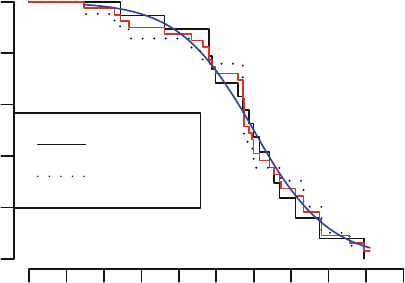
446 18 Parametric Survival Models

Residual

Survival Probability

−6 −5 −4 −3 −2 −1 0 1 2 3 4

0.0

0.2

0.4

0.6

0.8

1.0

Group 1

Group 2

Fig. 18.11 Kaplan–Meier estimates of distribution of standardized censored residu-

als from the log-logistic model, along with the assumed standard log-logistic distri-

bution (dashed curve). The step functions in red is the estimated distribution of all

residuals, and the step functions in black are the estimated distributions of residuals

stratiﬁed by group, as indicated. The blue curve is the assumed log-logistic distribu-

tion.

Section

19.2 has a more in-depth example of this approach.

18.3.7 Validating the Fitted Model

AFT models may be validated for both calibration and discrimination accu-

racy using the same methods that are presented for the Cox model in Sec-

tion

20.11. The methods discussed there for checking calibration are based on

choosing a single follow-up time. Checking the distributional assumptions of

the parametric model is also a check of calibration accuracy in a sense. An-

other indirect calibration assessment may be obtained from a set of Cox–Snell

residuals (Section

18.3.5) or by using ordinary residuals as just described. A

higher resolution indirect calibration assessment based on plotting individual

uncensored failure times is available when the theoretical censoring times for

those observations are known. Let C denote a subject’s censoring time and F

the cumulative distribution of a failure time T . The expected value of F (T |X)

is 0.5 when T is an actual failure time rando m variable. The expected value

for an event time that is observed because it is uncensored is the expected

value of F (T |T ≤ C, X)=0.5F (C|X). A smooth plot (using, say,

loess)of

F (T |X) − 0.5F (C|X) against X

β should b e a ﬂat line through y = 0 if the

model is well calibrated. A smooth plot of 2F (T |X)/F (C|X) against X

β (or

anything else) should be a ﬂat line through y = 1. This method assumes that

the model is calibrated well enough that we can substitute 1 −

S(C|X)for

F (C|X).

18.8 Time-Dependent Covariates 447

18.4 Buckley–James Regression Model

Buckley and James

developed a method for estima ting regression coeﬃ-

cients using least squares after imputing censored residuals. Their method

does not assume a distribution for surviva l time or the residuals, but is aimed

at estimating expected survival time or exp ected log survival time given pre-

dictor va riables. This method has been generalized to allow for smooth non-

linear eﬀects and interactions in the S

bj function in the rms package, written

by Stare and Harrell

585

18.5 Design Formulations

Va rious designs ca n be formulated with survival regression models just as

with other regressio n models. By constructing the proper dummy variables,

ANOVA and ANOCOVA models can easily be speciﬁed for testing diﬀerences

in survival time between multiple treatments. Interactions and complex non-

linear eﬀects may also be modeled.

18.6 Test Statistics

As discussed previously, likelihoo d ratio, score, and Wald statistics can be

derived from the maximum likelihood analysis, and the choice of test statistic

depends on the circumsta nce and on computational convenience.

18.7 Quantifying Predictive Ability

See Section

20.10 for a generalized measure of concordance between predicted

and observed survival time (or probability of survival) for right-censored data.

18.8 Time-Dependent Covariates

Time-dependent covariates (predictors) requires special likelihood functions

and add signiﬁcant complexity to analyses in exchange for greater ver-

satility and enhanced predictive discrimination

604

. Nicolaie et al.

477

and

D’Agostino et al.

145

provide useful static covariate approaches to modeling

time-dependent predictors using landmark analysis.

448 18 Parametric Survival Models

18.9 R Functions

Therneau’s survreg function (part of his survival package) can ﬁt regression

models in the AFT family with left–, right–, or interval–censoring. The time

variable can be untransformed or log-transformed (the default). Distributions

supported are extreme value (Weibull and expo nential), normal, logistic, and

Student-t. The version of survreg in rms that ﬁts parametric survival mo dels

in the same framework as lrm, ols,andcph is called psm. psm works with

print, coef, formula, specs, summary, anova, predict, Predict, fastbw, latex,

nomogram, validate, calibrate, survest,andsurvplot functions for obtaining

and plotting predicted surviva l probabilities. The dist argument to psm can be

"exponential", "extreme", "gaussian", "logistic", "loglogistic", "lognormal",

"t",or"weibull". To ﬁt a model with no covariables, use the command

psm(Surv(d.time , event ) ∼ 1)

To restate a Weibull or exponential model in PH form, use the pphsm function.

An example of how many of the functions are used is found below.

units(d.time ) ← "Year"

f ← psm(Surv(d.time ,cdeath ) ∼ lsp(age ,65)*sex)

# default is Weibull

anova(f)

summary(f) # summarize effects with delta log T

latex(f) # typeset math. form of fitted model

survest(f, times =1) # 1y survival est. for all subjects

survest(f, expand.grid (sex="female ", age=30:80) , times =1:2)

# 1y, 2y survival estimates vs. age, for females

survest(f, data.frame(sex="female ",age=50))

# survival curve for an individual subject

survplot(f, sex=NA, age=50, n.risk =T)

# survival curves for each sex, adjusting age to 50

f.ph ← pphsm (f) # convert from AFT to PH

summary(f.ph) # summarize with hazard ratios

# instead of changes in log(T)

Special functions work with objects created by psm to create S functions that

contain the analytic form for predicted survival probabilities (Survival), haz-

ard functions (Hazard), quantiles of survival time (Quantile), and mean or

expected survival time (Mean). Once the S functions are constructed, they can

be used in a variety of contexts. The survplot and survest functions have

a special argument for psm ﬁts: what. The default is what="survival" to esti-

mate or plot survival probabilities. Specifying what="hazard" will plot hazard

functions. Predict also has a special argument for psm ﬁts: time. Specifying a

single value for time results in survival probability for that time being plotted

instead of X

β. Examples of many of the functions appear below, with the

output of the survplot commandshowninFigure

18.12.

med ← Quantile(fl)

meant ← Mean(fl)

18.9 R Functions 449

haz ← Hazard (fl)

surv ← Survival(fl)

latex(surv , file= '', type= ' Sinput ' )

surv ← function (times = NULL , lp = NULL ,

parms = -2.15437773933124 )

{

1/(1 + exp((logb(times) - lp)/exp(parms )))

}

# Plot estimated hazard functions and add median

# survival times to graph

survplot(fl, group , what="hazard ") # Figure 18.12

# Compute median survival time

m ← med(lp=predict(fl,

data.frame(group=levels (kprats $group ))))

216.0857 240.0328

med(lp=range (fl$linear.predictors ))

[1] 216.0857 240.0328

m ← format (m, digits =3)

text(68, .02 , paste("Group 1 median : ", m[1],"\n",

"Group 2 median : ", m[2], sep=""))

# Compute survival probability at 210 days

xbeta ← predict(fl,

data.frame(group=c("Group 1","Group 2")))

surv(210, xbeta )

0.5612718 0.7599776

The S object called survreg.distributions in Therneau’s survival package

and the object survreg.auxinfo in the rms package have detailed information

for extreme-value, logistic, normal, and t distributions. For each distribution,

components include the deviance function, an algorithm for obtaining starting

parameter estimates, a L

X representation of the survival function, and S

functions deﬁning the surviva l, hazard, quantile functions, and basic survival

inverse function (which could have been used in Figure

18.9). See Figure 18.6

for examples. rms’s val.surv function is useful for indirect external valida-

tion of parametr ic models using Cox–Snell residuals and other approaches of

Section 18.3.7.Theplot metho d for an object created by val.surv makes it

easy to stratify all computations by a variable of interest to more stringently

valida te the ﬁt with respect to that variable.

rms’s bj function ﬁts the Buckley–James model for right-censored re-

sponses.

450 18 Parametric Survival Models

Days

Hazard Function

0 30 60 90 120 180 240 300

0.000

0.005

0.010

0.015

0.020

0.025

0.030

Group 1

Group 2

Group 1 median: 216

Group 2 median: 240

Fig. 18.12 Estimated hazard functions for log-logistic ﬁt to rat vaginal cancer data,

along with median survival times.

Kooperberg et al.’s adaptive linear spline log-hazard model

360, 361, 594

has

been implemented in the S function hare. Their procedure searches for second-

order interactions involving predictors (and linear splines of them) and linear

splines in follow-up time (allowing for non-proportional hazards). hare is also

used to estimate calibration curves for parametric survival models (rms func-

tion calibrate)asitisforCoxmodels.

18.10 Further Reading

Wellek

657

developed a test statistic for a speciﬁed maximum survival diﬀerence

after relating this diﬀerence to a hazard ratio.

Hougaard

308

compared accelerated failure time models with proportional haz-

ard models.

Gore et al.

226

discuss how an AFT model (the log-logistic model) giv es rise to

varying hazard ratios.

See Hillis

293

for other types of residuals and plots that use them.

SeeGoreetal.

226

and Lawless

382

for other methods of checking assumptions for

AFT models. Lawless is an excellent text for in-depth discussion of parametric

survival modeling. Kwong and Hutton

369

present other methods of choosing

parametric survival models, and discuss the robustness of estimates when ﬁtting

an incorrectly chosen accelerated failure time model.

18.11 Problems 451

18.11 Problems

1. For the failure times (in days)

133

compute MLEs of the following parameters of an exponential distribution

by hand: λ, μ, T

0.5

,andS(3 days). Compute 0.95 conﬁdence limits for λ

and S(3), basing the latter on log[Λ(t)].

2. For the same data in Problem 1, compute MLEs of parameters of a Weibull

distribution. Also compute the MLEs of S(3) and T

0.5

Chapter 19

Case Study in Parametric Survival

Modeling and Model Approximation

Consider the random sample of 1000 patients from the SUPPORT study,

352

described in Section 3.12. In this case study we develop a parametric sur-

vival time mo del (accelerated failure time model) for time until death for the

acute disease subset of SUPPORT (acute respiratory failure, multiple organ

system failure, coma). We eliminate the chronic disease categories because

the shapes of the survival curves are diﬀerent between acute and chronic dis-

ease categories. To ﬁt both acute and chronic disease classes would requir e a

log-normal model with σ pa rameter that is disease-speciﬁc.

Patients had to survive until day 3 of the study to qualify. The baseline

physiologic variables were measured during day 3.

19.1 Descriptive Statistics

First we create a variable acute to ﬂag the categories of interest, and print

univariable descriptive statistics for the data subset.

require(rms)

getHdata(support) # Get data frame from web site

acute ← support$dzclass %in% c( ' ARF/MOSF ' , ' Coma ' )

latex(describe(support[acute ,]), file= '')

F.E. Harrell, Jr., Regression Modeling Strategies, Springer Series

in Statistics, DOI 10.1007/978-3-319-19425-7

453

454 19 Parametric Survival Modeling and Model Approximation

support[acute, ]

35 Variables 537 Observations

age : Age

n missing unique Info Mean .05 .10 .25 .50 .75 .90 .95

537 0 529 1 60.7 28.49 35.22 47.93 63.67 74.49 81.54 85.56

lowest : 18.04 18.41 19.76 20.30 20.31

highest: 91.62 91.82 91.93 92.74 95.51

death : Death at any time up to NDI date:31DEC94

n missing unique Info Sum Mean

537 0 2 0.67 356 0.6629

sex

n missing unique

537 0 2

female (251, 47%), male (286, 53%)

hospdead : Death in Hospital

n missing unique Info Sum Mean

537 0 2 0.7 201 0.3743

slos : Days from Study Entry to Discharge

n missing unique Info Mean .05 .10 .25 .50 .75 .90 .95

537 0 85 1 23.44 4.0 5.0 9.0 15.0 27.0 47.4 68.2

lowest :34567,highest: 145 164 202 236 241

d.time : Days of Follow-Up

n missing unique Info Mean .05 .10 .25 .50 .75 .90 .95

537 0 340 1 446.1 4 6 16 182 724 1421 1742

lowest : 3 4 5 6 7, highest: 1977 1979 1982 2011 2022

dzgroup

n missing unique

537 0 3

ARF/MOSF w/Sepsis (391, 73%), Coma (60, 11%), MOSF w/Malig (86, 16%)

dzclass

n missing unique

537 0 2

ARF/MOSF (477, 89%), Coma (60, 11%)

num.co : number of comorbidities

n missing unique Info Mean

537 0 7 0.93 1.525

0 1 23456

Frequency 111 196 133 51 31 10 5

% 2136259621

19.1 Descriptive Statistics 455

edu : Years of Education

n missing unique Info Mean .05 .10 .25 .50 .75 .90 .95

411 126 22 0.96 12.03 7 8 10 12 14 16 17

lowest : 0 1 2 3 4, highest: 17 18 19 20 22

income

n missing unique

335 202 4

under $11k (158, 47%), $11-$25k (79, 24%), $25-$50k (63, 19%)

>$50k (35, 10%)

scoma : SUPPORT Coma Score based on Glasgow D3

n missing unique Info Mean .05 .10 .25 .50 .75 .90 .95

537 0 11 0.82 19.24 0 0 0 0 37 55 100

0 9 26 37 41 44 55 61 89 94 100

Frequency 301 50 44 19 17 43 11 6 8 6 32

% 56984382111 6

charges : Hospital Charges

n missing unique Info Mean .05 .10 .25 .50 .75 .90 .95

517 20 516 1 86652 11075 15180 27389 51079 100904 205562 283411

lowest : 3448 4432 4574 5555 5849

highest: 504660 538323 543761 706577 740010

totcst : Total RCC cost

n missing unique Info Mean .05 .10 .25 .50 .75 .90 .95

471 66 471 1 46360 6359 8449 15412 29308 57028 108927 141569

lowest : 0 2071 2522 3191 3325

highest: 269057 269131 338955 357919 390460

totmcst : Total micro-cost

n missing unique Info Mean .05 .10 .25 .50 .75 .90 .95

331 206 328 1 39022 6131 8283 14415 26323 54102 87495 111920

lowest : 0 1562 2478 2626 3421

highest: 144234 154709 198047 234876 271467

avtisst : Average TISS, Days 3–25

n missing unique Info Mean .05 .10 .25 .50 .75 .90 .95

536 1 205 1 29.83 12.46 14.50 19.62 28.00 39.00 47.17 50.37

lowest : 4.000 5.667 8.000 9.000 9.500

highest: 58.500 59.000 60.000 61.000 64.000

race

n missing unique

535 2 5

white black asian other hispanic

Frequency 417 84 4 8 22

% 781611 4

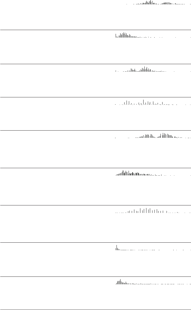
456 19 Parametric Survival Modeling and Model Approximation

meanbp : Mean Arterial Blood Pressure Day 3

n missing unique Info Mean .05 .10 .25 .50 .75 .90 .95

537 0 109 1 83.28 41.8 49.0 59.0 73.0 111.0 124.4 135.0

lowest : 0 20 27 30 32, highest: 155 158 161 162 180

wblc : White Blood Cell Count Day 3

n missing unique Info Mean .05 .10 .25 .50 .75 .90 .95

532 5 241 1 14.1 0.8999 4.5000 7.9749 12.3984 18.1992 25.1891 30.1873

lowest : 0.05000 0.06999 0.09999 0.14999 0.19998

highest: 51.39844 58.19531 61.19531 79.39062 100.00000

hrt : Heart Rate Day 3

n missing unique Info Mean .05 .10 .25 .50 .75 .90 .95

537 0 111 1 105 51 60 75 111 126 140 155

lowest : 0 11 30 36 40, highest: 189 193 199 232 300

resp : Respiration Rate Day 3

n missing unique Info Mean .05 .10 .25 .50 .75 .90 .95

537 0 45 1 23.72 8 10 12 24 32 39 40

lowest : 0 4 6 7 8, highest: 48 49 52 60 64

temp : Temperature (celcius) Day 3

n missing unique Info Mean .05 .10 .25 .50 .75 .90 .95

537 0 61 1 37.52 35.50 35.80 36.40 37.80 38.50 39.09 39.50

lowest : 32.50 34.00 34.09 34.90 35.00

highest: 40.20 40.59 40.90 41.00 41.20

paﬁ : PaO2/(.01*FiO2) Day 3

n missing unique Info Mean .05 .10 .25 .50 .75 .90 .95

500 37 357 1 227.2 86.99 105.08 137.88 202.56 290.00 390.49 433.31

lowest : 45.00 48.00 53.33 54.00 55.00

highest: 574.00 595.12 640.00 680.00 869.38

alb : Serum Albumin Day 3

n missing unique Info Mean .05 .10 .25 .50 .75 .90 .95

346 191 34 1 2.668 1.700 1.900 2.225 2.600 3.100 3.400 3.800

lowest : 1.100 1.200 1.300 1.400 1.500

highest: 4.100 4.199 4.500 4.699 4.800

bili : Bilirubin Day 3

n missing unique Info Mean .05 .10 .25 .50 .75 .90 .95

386 151 88 1 2.678 0.3000 0.4000 0.6000 0.8999 2.0000 6.5996 13.1743

lowest : 0.09999 0.19998 0.29999 0.39996 0.50000

highest: 22.59766 30.00000 31.50000 35.00000 39.29688

crea : Serum creatinine Day 3

n missing unique Info Mean .05 .10 .25 .50 .75 .90 .95

537 0 84 1 2.232 0.6000 0.7000 0.8999 1.3999 2.5996 5.2395 7.3197

lowest : 0.3 0.4 0.5 0.6 0.7, highest: 10.4 10.6 11.2 11.6 11.8

19.1 Descriptive Statistics 457

sod : Serum sodium Day 3

n missing unique Info Mean .05 .10 .25 .50 .75 .90 .95

537 0 38 1 138.1 129 131 134 137 142 147 150

lowest : 118 120 121 126 127, highest: 156 157 158 168 175

ph : Serum pH (arterial) Day 3

n missing unique Info Mean .05 .10 .25 .50 .75 .90 .95

500 37 49 1 7.416 7.270 7.319 7.380 7.420 7.470 7.510 7.529

lowest : 6.960 6.989 7.069 7.119 7.130

highest: 7.560 7.569 7.590 7.600 7.659

glucose : Glucose Day 3

n missing unique Info Mean .05 .10 .25 .50 .75 .90 .95

297 240 179 1 167.7 76.0 89.0 106.0 141.0 200.0 292.4 347.2

lowest : 30 42 52 55 68, highest: 446 468 492 576 598

bun : BUN Day 3

n missing unique Info Mean .05 .10 .25 .50 .75 .90 .95

304 233 100 1 38.91 8.00 11.00 16.75 30.00 56.00 79.70 100.70

lowest :13456,highest: 123 124 125 128 146

urine : Urine Output Day 3

n missing unique Info Mean .05 .10 .25 .50 .75 .90 .95

303 234 262 1 2095 20.3 364.0 1156.5 1870.0 2795.0 4008.6 4817.5

lowest : 0 5 8 15 20, highest: 6865 6920 7360 7560 7750

adlp : ADL Patient Day 3

n missing unique Info Mean

104 433 8 0.87 1.577

0 1234567

Frequency 51 19 7 6 4 7 8 2

% 4918764782

adls : ADL Surrogate Day 3

n missing unique Info Mean

392 145 8 0.89 1.86

01234567

Frequency 185 68 22 18 17 20 39 23

% 47176545106

sfdm2

n missing unique

468 69 5

no(M2 and SIP pres) (134, 29%), adl>=4 (>=5 if sur) (78, 17%)

SIP>=30 (30, 6%), Coma or Intub (5, 1%), <2 mo. follow-up (221, 47%)

458 19 Parametric Survival Modeling and Model Approximation

adlsc : Imputed ADL Calibrated to Surrogate

n missing unique Info Mean .05 .10 .25 .50 .75 .90 .95

537 0 144 0.96 2.119 0.000 0.000 0.000 1.839 3.375 6.000 6.000

lowest : 0.0000 0.4948 0.4948 1.0000 1.1667

highest: 5.7832 6.0000 6.3398 6.4658 7.0000

Next, patterns of missing data are displayed.

plot(naclus (support[acute ,])) # Figure 19.1

The Hmisc varclus function is used to quantify and depict associations between

predictors, allowing for general nonmonotonic relatio nships. This is done by

using Hoeﬀding’s D as a similarity measure for all possible pairs of predictors

instead of the default similarity, Spearman’s ρ.

ac ← support[acute ,]

ac$dzgroup ← ac$dzgroup[drop=TRUE] # Remove unused levels

label(ac$dzgroup ) ← ' Disease Group '

attach(ac)

vc ← varclus(∼ age + sex + dzgroup + num.co + edu + income +

scoma + race + meanbp + wblc + hrt + resp +

temp + pafi + alb + bili + crea + sod + ph +

glucose + bun + urine + adlsc , sim= ' hoeffding ' )

plot(vc) # Figure 19.2

19.2 Checking Adequacy of Log-Normal Accelerated

Failure Time Model

Let us check whether a parametric survival time model will ﬁt the data, with

respect to the key prognostic factors. First, Kaplan–Meier estimates stratiﬁed

by disease group are computed, and plotted after inverse normal transforma-

tion, against log t. Parallelism and linearity indica te goodness of ﬁt to the

log normal distribution for disease group. Then a more stringent assessment

is made by ﬁtting an initial model and computing right-censored residuals.

These residuals, after dividing by ˆσ, should all have a normal distribution

if the model holds. We compute Kaplan–Meier estimates of the distribution

of the residuals and overlay the estimated survival distribution with the the-

oretical Gaussian one. This is done overall, and then to get more stringent

assessments of ﬁt, residuals are stratiﬁed by key predictors and plots are

produced that contain multiple Kaplan–Meier curves along with a single the-

oretical normal curve. All curves should hover about the normal distribution.

To gauge the natural variability of stratiﬁed residual distribution estimates,

the residuals are also stratiﬁed by a random number that has no bearing on

the goodness of ﬁt.

dd ← datadist(ac)

# describe distributions of variables to rms

19.2 Checking Adequacy of Log-Normal Model 459

adlsc

sod

crea

temp

resp

hrt

meanbp

race

avtisst

wblc

charges

totcst

scoma

pafi

sfdm2

alb

bili

totmcst

adlp

urine

glucose

bun

adls

edu

income

num.co

dzclass

dzgroup

d.time

slos

hospdead

sex

age

death

0.5

0.4

0.3

0.2

0.1

0.0

Fraction Missing

Fig. 19.1 Cluster analysis showing which predictors tend to be missing on the same

patients

raceasian

raceother

racehispanic

raceblack

urine

glucose

bun

num.co

adlsc

resp

hrt

temp

meanbp

pafi

alb

bili

age

crea

edu

income$11−$25k

income$25−$50k

income>$50k

sexmale

sod

dzgroupComa

scoma

dzgroupMOSF w/Malig

wblc

0.20

0.15

0.10

0.05

0.00

30 * Hoeffding D

Fig. 19.2 Hierarchical clustering of potential predictors using Hoeﬀding D as a

similarity measure. Categorical predictors are automatically expanded into dummy

variables.

options(datadist= ' dd ' )

# Generate right-censored survival time variable

years ← d.time /365.25

units(years) ← ' Year '

S ← Surv(years , death)

# Show normal inverse Kaplan-Meier estimates

# stratified by dzgroup

survplot(npsurv (S ∼ dzgroup), conf= ' none ' ,

fun=qnorm ,logt=TRUE) # Figure 19.3

460 19 Parametric Survival Modeling and Model Approximation

f ← psm (S ∼ dzgroup + rcs(age ,5) + rcs(meanbp ,5),

dist= ' lognormal ' , y=TRUE)

r ← resid(f)

survplot (r, dzgroup , label.curve =FALSE)

survplot (r, age, label.curve =FALSE)

survplot (r, meanbp , label.curve =FALSE)

random ← runif(length(age)); label(random) ← ' Random Number '

survplot (r, random , label.curve =FALSE) # Fig. 19.4

Now remove from consideration predictors that are missing in more than 0.2

of patients. Many of these were collected only for the second half of SUP-

PORT. Of those variables to be included in the model, ﬁnd which ones have

enough potential predictive power to justify allowing for nonlinear relation-

ships or multiple categories, which spe nd more d.f. For each va riable compute

Spearman ρ

based on multiple linear regression of rank(x), rank(x)

,andthe

log Survival Time in Years

−3

−2 −1 0 1 2

−2

−1

dzgroup=ARF/MOSF w/Sepsis

dzgroup=Coma

dzgroup=MOSF w/Malig

Fig. 19.3 Φ

−1

(t)) stratiﬁed by dzgroup. Linearity and semi-parallelism indi-

cate a reasonable ﬁt to the log-normal accelerated failure time model with respect to

one predictor.

surviva l time, truncating survival time at the shortest follow-up for survivor s

(356 days; see Section

4.1).

shortest.follow.up ← min(d.time [death ==0], na.rm =TRUE)

d.timet ← pmin(d.time , shortest.follow.up )

w ← spearman2(d.timet ∼ age + num.co + scoma + meanbp +

hrt + resp + temp + crea + sod + adlsc +

wblc + pafi + ph + dzgroup + race , p=2)

plot(w, main= '') # Figure 19.5

19.2 Checking Adequacy of Log-Normal Model 461

A b etter approach is to use the complete information in the failure and censor-

ing times by computing Somers’ D

rank correlation allowing for censoring.

w ← rcorrcens (S ∼ age + num.co + scoma + meanbp + hrt + resp +

temp + crea + sod + adlsc + wblc + pafi + ph +

dzgroup + race)

plot(w, main= '') # Figure 19.6

Remaining missing values are imputed using the “most normal” values, a

procedure found to work adequately for this particular study. Race is imputed

using the modal category.

# Compute number of missing values per variable

sapply (llist(age ,num.co ,scoma ,meanbp ,hrt ,resp ,temp ,crea ,sod ,

adlsc ,wblc ,pafi ,ph), function(x) sum(is.na (x)))

age num.co scoma meanbp hrt resp temp crea sod adlsc

0000000000

wblc pafi ph

53737

Residual

Survival Probability

−3.0 −2.0 −1.0 0.0 0.5 1.0 1.5 2.0

0.0

0.2

0.4

0.6

0.8

1.0

Disease Group

Residual

Survival Probability

−3.0 −2.0 −1.0 0.0 0.5 1.0 1.5 2.0

0.0

0.2

0.4

0.6

0.8

1.0

Age

Residual

Survival Probability

−3.0 −2.0 −1.0 0.0 0.5 1.0 1.5 2.0

0.0

0.2

0.4

0.6

0.8

1.0

Mean Arterial Blood Pressure Day 3

Residual

Survival Probability

−3.0 −2.0 −1.0 0.0 0.5 1.0 1.5 2.0

0.0

0.2

0.4

0.6

0.8

1.0

Random Number

Fig. 19.4 Kaplan-Meier estimates of distributions of normalized, right-censored

residuals from the ﬁtted log-normal surviv al model. Residuals are stratiﬁed by im-

portant variables in the mo del (by quartiles of continuous variables), plus a random

variable to depict the natural variability (in the lower right plot). Theoretical standard

Gaussian distributions of residuals are shown with a thick solid line.

462 19 Parametric Survival Modeling and Model Approximation

scoma

meanbp

dzgroup

crea

pafi

sod

hrt

adlsc

temp

wblc

num.co

age

resp

race

N df

535 4

537 2

532 2

537 2

500 2

537 2

0.00 0.02 0.04 0.06 0.08 0.10 0.12

Adjusted ρ

Fig. 19.5 Generalized Spearman ρ

rank correlation between predictors and trun-

cated survival time

meanbp

crea

dzgroup

scoma

pafi

adlsc

age

num.co

hrt

resp

race

sod

wblc

temp

537

532

537

535

537

500

537

0.00 0.05 0.10 0.15 0.20

Fig. 19.6 Somers’ D

rank correlation between predictors and original survival

time. For dzgroup or race, the correlation coeﬃcient is the maximum correlation from

using a dummy variable to represent the most frequent or one to represent the second

most frequent category.’,scap=’Somers’ D

rank correlation between predictors and

original survival time

19.2 Checking Adequacy of Log-Normal Model 463

# Can also do naplot(naclus(support[acute ,]))

# Can also use the Hmisc naclus and naplot functions

# Impute missing values with normal or modal values

wblc.i ← impute (wblc , 9)

pafi.i ← impute (pafi , 333.3)

ph.i ← impute (ph, 7.4)

race2 ← race

levels (race2) ← list(white = ' white ' ,other =levels (race)[-1])

race2[is.na(race2 )] ← ' white '

dd ← datadist(dd, wblc.i , pafi.i , ph.i , race2 )

Now that missing values have been imputed, a formal multivariable redun-

dancy analysis can be undertaken. The Hmisc package’s redun function goes

farther than the varclus pairwise correlation approach and allows for non-

monotonic transformations in predicting each predictor from all the others.

redun(∼ crea + age + sex + dzgroup + num.co + scoma + adlsc +

race2 + meanbp + hrt + resp + temp + sod + wblc.i +

pafi.i + ph.i, nk=4)

Redundancy Analysis

redun(formula = ∼crea + age + sex + dzgroup + num.co + scoma +

adlsc + race2 + meanbp + hrt + resp + temp + sod + wblc.i +

pafi.i + ph.i, nk = 4)

n: 537 p: 16 nk: 4

Number of NAs: 0

Transformation of target variables forced to be linear

cutoff: 0.9 Type: ordinary

with which each variable can be predicted from all other variables:

crea age sex dzgroup num.co scoma adlsc race2 meanbp

0.133 0.246 0.132 0.451 0.147 0.418 0.153 0.151 0.178

hrt resp temp sod wblc.i pafi.i ph.i

0.258 0.131 0.197 0.135 0.093 0.143 0.171

No redundant variables

Now turn to a more eﬃcient approach for gauging the p otential of each

predictor, one that makes maximal use of failure time and censored data is to

all continuous variables to have a maximum number of knots in a log-normal

surviva l model. This approach must use imputation to have an adequate

sample size. A semi-saturated main eﬀects additive log-normal model is ﬁtted.

It is necessary to limit restricted cubic splines to 4 knots, force

scoma to be

linear, and to omit ph.i in order to avoid a singular covariance matrix in

the ﬁt.

k ← 4

f ← psm(S ∼ rcs(age ,k)+sex+dzgroup+pol(num.co ,2)+scoma +

pol(adlsc ,2)+ race+rcs(meanbp ,k)+rcs(hrt ,k)+

464 19 Parametric Survival Modeling and Model Approximation

rcs(resp ,k)+rcs(temp ,k)+ rcs(crea ,3)+ rcs(sod ,k)+

rcs(wblc.i ,k)+rcs(pafi.i ,k), dist= ' lognormal ' )

plot(anova (f)) # Figure 19.7

Figure 19.7 properly blinds the analyst to the form of eﬀects (tests of lin-

earity). Next ﬁt a log-normal survival model with number of parameters

corresponding to nonlinear eﬀects determined from the partial χ

tests in

Figure

19.7. For the most promising predictors, ﬁve knots can be allocated,

as there are fewer singularity problems once less promising predictors a re

simpliﬁed.

sex

temp

race

sod

num.co

hrt

wblc.i

adlsc

resp

scoma

pafi.i

age

meanbp

crea

dzgroup

0102030

− df

Fig. 19.7 Partial χ

statistics for association of each predictor with response from

saturated main eﬀects model, penalized for d.f.

f ← psm(S ∼ rcs(age ,5)+ sex+dzgroup+num.co +

scoma+pol(adlsc ,2)+ race2+rcs(meanbp ,5)+

rcs(hrt ,3)+rcs(resp ,3)+temp+

rcs(crea ,4)+ sod+rcs(wblc.i ,3)+rcs(pafi.i ,4),

dist= ' lognormal ' )

print(f, latex =TRUE , coefs=FALSE)

Parametric Survival Model: Log Normal Distribution

psm(formula = S ~ rcs(age, 5) + sex + dzgroup + num.co + scoma +

pol(adlsc, 2) + race2 + rcs(meanbp, 5) + rcs(hrt, 3) + rcs(resp,

3) + temp + rcs(crea, 4) + sod + rcs(wblc.i, 3) + rcs(pafi.i,

4), dist = "lognormal")

19.2 Checking Adequacy of Log-Normal Model 465

Model Likelihood Discrimination

Ratio Test Indexes

Obs 537 LR χ

236.83 R

0.594

Events 356 d.f. 30 D

0.485

σ 2.230782 Pr(>χ

) < 0.0001 g 0.033

1.959

a ← anova (f)

Table 19.1 Wald Statistics for S

d.f. P

age 15.99 4 0.0030

Nonlinear 0.23 3 0.9722

sex 0.11 1 0.7354

dzgroup 45.69 2 < 0.0001

num.co 4.99 1 0.0255

scoma 10.58 1 0.0011

adlsc 8.28 2 0.0159

Nonlinear 3.31 1 0.0691

race2 1.26 1 0.2624

meanbp 27.62 4 < 0.0001

Nonlinear 10.51 3 0.0147

hrt 11.83 2 0.0027

Nonlinear 1.04 1 0.3090

resp 11.10 2 0.0039

Nonlinear 8.56 1 0.0034

temp 0.39 1 0.5308

crea 33.63 3 < 0.0001

Nonlinear 21.27 2 < 0.0001

so d 0.08 1 0.7792

wblc.i 5.47 2 0.0649

Nonlinear 5.46 1 0.0195

paﬁ.i 15.37 3 0.0015

Nonlinear 6.97 2 0.0307

TOTAL NONLINEAR 60.48 14 < 0.0001

TOTAL 261

.47 30 < 0.0001

466 19 Parametric Survival Modeling and Model Approximation

19.3 Summarizing the Fitted Model

First let’s plot the shape of the eﬀect of each predictor on log surviva l time.

All eﬀects are centered so that they can b e placed on a common scale. This

allows the relative strength of various predictors to be judged. Then Wald

statistics, penalized for d.f., are plotted in descending order. Next, rela-

tive eﬀects of varying predictors over reasonable ranges (survival time ratios

varying continuous predictors from the ﬁrst to the third quartile) are charted.

ggplot (Predict(f, ref.zero=TRUE), vnames = ' names ' ,

sepdiscrete= ' vertical ' , anova =a) # Figure 19.8

latex(a, file= '',label= ' tab:support-anovat ' ) # Table 19.1

plot(a) # Figure 19.9

options(digits =3)

plot(summary(f), log=TRUE , main= '') # Figure 19.10

19.4 Internal Validation of the Fitted Model

Using the Bootstrap

Let us decide whether there was signiﬁcant overﬁtting during the development

of this model, using the bootstrap.

# First add data to model fit so bootstrap can re-sample

# from the data

g ← update (f, x=TRUE , y=TRUE)

set.seed(717)

latex(validate(g, B=300), digits =2, size= ' Ssize ' )

Index Original Training Test O ptimism Co rrected n

Sample Sample Sample Index

0.49 0.51 0.46 0.05 0.43 300

0.59 0.66 0.54 0.12 0.47 300

Intercept 0.00 0.00 −0.05 0.05 −0.05 300

Slope 1.00 1.00 0.90 0.10 0.90 300

D 0.48 0.55 0.42 0.13 0.35 300

U 0.00 0.00 −0.01 0.01 −0.01 300

Q 0.48 0.56 0.43 0.12 0.36 300

g 1.96 2.05 1.87 0.19 1.77 300

19.4 Internal Validation of the Fitted Model Using the Bootstrap 467

= 8.3

= 16

= 33.6

= 11.8

= 27.6

= 5

= 15.4

= 11.1

= 10.6

= 0.1

= 0.4

= 5.5

adlsc age crea hrt

meanbp num.co pafi.i resp

scoma sod temp wblc.i

−3

−2

−1

−3

−2

−1

−3

−2

−1

024620 40 60 80 2.5 5.0 7.5 50 100 150

30 60 90 120 1500246100 200 300 400 500 10 20 30 40

0 25 50 75 100 130 135 140 145 150155 35 36 37 38 39 40 010203040

log(T)

= 45.7

= 1.3

= 0.1

ARF/MOSF w/Sepsis

Coma

MOSF w/Malig

white

other

female

male

−3 −2 −1 0 1 2 −3 −2 −1 0 1 2 −3 −2 −1 0 1 2

log(T)

dzgroup race2 sex

Fig. 19.8 Eﬀect of each predictor on log survival time. Predicted values have been

centered so that predictions at predictor reference values are zero. Pointwise 0.95

conﬁdence bands are also shown. As all y-axes have the same scale, it is easy to see

which predictors are strongest.

Judging from D

and R

there is a moderate amount of overﬁtting. The

slope shrinkage factor (0.9) is not troublesome, however. An almost unbiased

estimate o f future predictive discrimination on similar patients is given by

the corrected D

of 0.43. This index equals the diﬀerence between the prob-

ability of concordance and the probability of disco rdance of pairs of predicted

survival times and pairs of observed survival times, accounting for censoring.

Next, a b ootstrap overﬁtting-corrected calibration curve is estimated. Pa-

tients are stratiﬁed by the predicted probability of surviving one year, such

that there are at least 60 patients in each group.

468 19 Parametric Survival Modeling and Model Approximation

sod

sex

temp

race2

wblc.i

num.co

adlsc

resp

scoma

hrt

age

pafi.i

meanbp

crea

dzgroup

0 10203040

− df

Fig. 19.9 Contribution of variables in predicting survival time in log-normal model

0.10 0.50 1.00 2.00 3.50

age − 74.5:47.9

num.co − 2:1

scoma − 37:0

adlsc − 3.38:0

meanbp − 111:59

hrt − 126:75

resp − 32:12

temp − 38.5:36.4

crea − 2.6:0.9

sod − 142:134

wblc.i − 18.2:8.1

pafi.i − 323:142

sex − female:male

dzgroup − Coma:ARF/MOSF w/Sepsis

dzgroup − MOSF w/Malig:ARF/MOSF w/Sepsis

race2 − other:white

Fig. 19.10 Estimated survival time ratios for default settings of predictors. For

example, when age changes from its lower quartile to the upper quartile (47.9y to

74.5y), median surviv al time decreases by more than half. Diﬀerent shaded areas of

bars indicate diﬀerent conﬁdence levels (.9, 0.95, 0.99).

set.seed(717)

cal ← calibrate(g, u=1, B=300)

plot(cal , subtitles=FALSE)

cal ← calibrate(g, cmethod= ' KM ' , u=1, m=60, B=120, pr=FALSE)

plot(cal , add=TRUE) # Figure 19.11

19.5 Approximating the Full Model 469

0.0 0.2 0.4 0.6 0.8

0.0

0.2

0.4

0.6

0.8

Predicted 1 Year Survival

Fraction Surviving 1 Years

Fig. 19.11 Bootstrap validation of calibration curve. Dots represent apparent cali-

bration accuracy; × are bootstrap estimates corrected for overﬁtting, based on bin-

ning predicted survival probabilities and computing Kaplan-Meier estimates. Black

curve is the estimated observed relationship using hare and the blue curve is the

o verﬁtting-corrected hare estimate. The gray-scale line depicts the ideal relationship.

19.5 Approximating the Full Model

The ﬁtted log-normal model is perhaps too complex for routine use and for

routine data collection. Let us develop a simpliﬁed model that can predict

the predicted values of the full model with high accuracy (R

=0.967). The

simpliﬁcation is done using a fast backward step-down against the full model

predicted values.

Z ← predict(f) #X* beta hat

a ← ols(Z ∼ rcs(age ,5)+ sex+dzgroup+num.co +

scoma+pol(adlsc ,2)+ race2+

rcs(meanbp ,5)+rcs(hrt ,3)+ rcs(resp ,3)+

temp+rcs(crea ,4)+sod+rcs(wblc.i ,3)+

rcs(pafi.i ,4), sigma =1)

# sigma=1 is used to prevent sigma hat from being zero when

# R2=1.0 since we start out by approximating Z with all

# component variables

fastbw (a, aics =10000) # fast backward stepdown

Deleted Chi-Sq d.f. P Residual d.f. P AIC R2

sod 0.43 1 0.512 0.43 1 0.5117 -1.57 1.000

sex 0.57 1 0.451 1.00 2 0.6073 -3.00 0.999

temp 2.20 1 0.138 3.20 3 0.3621 -2.80 0.998

race2 6.81 1 0.009 10.01 4 0.0402 2.01 0.994

wblc.i 29.52 2 0.000 39.53 6 0.0000 27.53 0.976

470 19 Parametric Survival Modeling and Model Approximation

num.co 30.84 1 0.000 70.36 7 0.0000 56.36 0.957

resp 54.18 2 0.000 124.55 9 0.0000 106.55 0.924

adlsc 52.46 2 0.000 177.00 11 0.0000 155.00 0.892

pafi.i 66.78 3 0.000 243.79 14 0.0000 215.79 0.851

scoma 78.07 1 0.000 321.86 15 0.0000 291.86 0.803

hrt 83.17 2 0.000 405.02 17 0.0000 371.02 0.752

age 68.08 4 0.000 473.10 21 0.0000 431.10 0.710

crea 314.47 3 0.000 787.57 24 0.0000 739.57 0.517

meanbp 403.04 4 0.000 1190.61 28 0.0000 1134.61 0.270

dzgroup 441.28 2 0.000 1631.89 30 0.0000 1571.89 0.000

Approximate Estimates after Deleting Factors

Coef S.E. Wald Z P

[1,] -0.5928 0.04315 -13.74 0

Factors in Final Model

None

f.approx ← ols(Z ∼ dzgroup + rcs(meanbp ,5) + rcs(crea ,4) +

rcs(age ,5) + rcs(hrt ,3) + scoma +

rcs(pafi.i ,4) + pol(adlsc ,2)+

rcs(resp ,3), x=TRUE)

f.approx$stats

n Model L.R. d.f. R2 g Sigma

537.000 1688.225 23.000 0.957 1.915 0.370

We can estimate the variance–covariance matrix of the coeﬃcients of the

reduced model using Equation 5.2 in Section 5.5.2. The computations below

result in a covariance matrix that does no t include elements related to the

scale parameter. In the co de x is the matrix T in Section

5.5.2.

V ← vcov(f,regcoef.only=TRUE) # var(full model)

X ← cbind (Intercept=1, g$x) # full model design

x ← cbind (Intercept=1, f.approx$x) # approx. model design

w ← solve (t(x) %*% x, t(x)) %*% X # contrast matrix

v ← w %*% V %*% t(w)

Let’s compare the variance estimates (diagonals o f v) with variance estimates

from a reduced model that is ﬁtted against the actual outcomes.

f.sub ← psm(S ∼ dzgroup + rcs(meanbp ,5) + rcs(crea ,4) +

rcs(age ,5) + rcs(hrt ,3) + scoma + rcs(pafi.i ,4) +

pol(adlsc ,2)+ rcs(resp ,3), dist= ' lognormal ' )

diag(v)/diag(vcov(f.sub,regcoef.only=TRUE))

Intercept dzgroup=Coma dzgroup=MOSF w/Malig

0.981 0.979 0.979

meanbp meanbp ' meanbp ''

0.977 0.979 0.979

meanbp ''' crea crea '

0.979 0.979 0.979

crea '' age age '

0.979 0.982 0.981

age '' age ''' hrt

0.981 0.980 0.978

19.5 Approximating the Full Model 471

hrt ' scoma pafi.i

0.976 0.979 0.980

pafi.i ' pafi.i '' adlsc

0.980 0.980 0.981

adlsc

∧

2 resp resp '

0.981 0.978 0.977

r ← diag(v)/diag(vcov(f.sub ,regcoef.only =TRUE ))

r[c(which.min(r), which.max(r))]

hrt ' age

0.976 0.982

The estimated variances from the reduced model are actually slightly smaller

than those that would have been obtained from stepwise variable selection

in this ca se, had variable selectio n used a stopping rule that resulted in the

same set of variables being selected. Now let us compute Wald statistics for

the reduced model.

f.approx$var ← v

latex(anova(f.approx , test= ' Chisq ' , ss=FALSE ), file= '',

label= ' tab:support-anovaa ' )

The results are shown in Table 19.2. Note the similarity of the statistics

to those found in the table for the full model. This would not be the case had

deleted variables been very collinear with retained variables.

The equation for the simpliﬁed model follows. The model is also depicted

graphically in Figure

19.12. The nomogram allows one to calculate mean and

median survival time. Survival probabilities could have easily been added as

additional axes.

# Typeset mathematical form of approximate model

latex(f.approx , file= '')

E(Z) = Xβ, where

β =

−2.51

−1.94[Coma] − 1.75[MOSF w/Malig]

+0.068meanbp − 3.08×10

−5

(meanbp − 41.8)

+7.9×10

−5

(meanbp − 61)

−4.91×10

−5

(meanbp − 73)

+2.61×10

−6

(meanbp − 109)

− 1.7×10

−6

(meanbp − 135)

−0.553crea − 0.229(crea − 0.6)

+0.45(crea − 1.1)

− 0.233(crea − 1.94)

+0.0131(crea − 7.32)

−0.0165age − 1.13×10

−5

(age − 28.5)

+4.05×10

−5

(age − 49.5)

−2.15×10

−5

(age − 63.7)

− 2.68×10

−5

(age − 72.7)

+1.9×10

−5

(age − 85.6)

−0.0136hrt + 6.09×10

−7

(hrt − 60)

− 1.68×10

−6

(hrt − 111)

+1.07×10

−6

(hrt − 140)

−0.0135 scoma

+0.0161paﬁ.i − 4.77×10

−7

(paﬁ.i − 88)

+9.11×10

−7

(paﬁ.i − 167)

472 19 Parametric Survival Modeling and Model Approximation

Table 19.2 Wald Statistics for Z

d.f. P

dzgroup 55.94 2 < 0.0001

meanbp 29.87 4 < 0.0001

Nonlinear 9.84 3 0.0200

crea 39.04 3 < 0.0001

Nonlinear 24.37 2 < 0.0001

age 18.12 4 0.0012

Nonlinear 0.34 3 0.9517

hrt 9.87 2 0.0072

Nonlinear 0.40 1 0.5289

scoma 9.85 1 0.0017

paﬁ.i 14.01 3 0.0029

Nonlinear 6.66 2 0.0357

adlsc 9.71 2 0.0078

Nonlinear 2.87 1 0.0904

resp 9.65 2 0.0080

Nonlinear 7.13 1 0.0076

TOTAL NONLINEAR 58.08 13 < 0.0001

TOTAL 252.32 23 < 0.0001

−5.02×10

−7

(paﬁ.i − 276)

+6.76×10

−8

(paﬁ.i − 426)

− 0.369 adlsc + 0.0409 adlsc

+0.0394resp − 9.11×10

−5

(resp − 10)

+0.000176(resp − 24)

− 8.5×10

−5

(resp − 39)

and [c] = 1 if subject is in group c, 0otherwise; (x)

= x if x>0, 0

otherwise.

# Derive S functions that express mean and quantiles

# of survival time for specific linear predictors

# analytically

expected.surv ← Mean(f)

quantile.surv ← Quantile(f)

latex(expected.surv , file= '', type= ' Sinput ' )

expected.surv ← function (lp = NULL ,

parms = 0.802352037606488 )

{

names(parms) ← NULL

exp(lp + exp(2 * parms)/2)

}

latex(quantile.surv , file= '', type= ' Sinput ' )

quantile.surv ← function (q = 0.5, lp = NULL ,

parms = 0.802352037606488 )

19.6 Problems 473

{

names(parms) ← NULL

f ← function(lp, q, parms) lp + exp(parms ) * qnorm(q)

names(q) ← format (q)

drop(exp(outer (lp, q, FUN = f, parms = parms )))

}

median.surv ← function(x) quantile.surv (lp=x)

# Improve variable labels for the nomogram

f.approx ← Newlabels (f.approx , c( ' Disease Group ' ,

' Mean Arterial BP ' , ' Creatinine ' , ' Age ' , ' Heart Rate ' ,

' SUPPORT Coma Score ' , ' PaO2/(.01*FiO2) ' , ' ADL ' ,

' Resp. Rate ' ))

nom ←

nomogram (f.approx ,

pafi.i=c(0, 50, 100, 200, 300, 500, 600, 700, 800,

900),

fun=list( ' Median Survival Time ' =median.surv ,

' Mean Survival Time ' =expected.surv),

fun.at=c(.1,.25,.5,1,2,5,10,20,40))

plot(nom , cex.var=1, cex.axis =.75, lmgp=.25)

# Figure 19.12

19.6 Problems

Analyze the Mayo Clinic PBC dataset.

1. Graphically assess whether Weibull (extreme value), exponential, log-

logistic, or log-normal distr ibutions will ﬁt the data, using a few apparently

important stratiﬁcation factors.

2. For the best ﬁtting parametric model from among the four examined,

ﬁt a model containing several sensible covariables, both categorical and

continuous. Do a Wa ld test for whether each factor in the model has an

association with survival time, and a likelihood ratio test for the simulta-

neous contribution of all pr edictors. For classiﬁcation factors having more

than two levels, be sure that the Wald test has the appropriate degrees

of freedom. For continuous factors, verify or relax linearity assumptions.

If using a Weibull model, test whether a simpler exponential model would

be appropriate. Interpret all estimated coeﬃcients in the model. Write the

full survival model in mathematica l form. Generate a predicted survival

curve for a patient with a given set of characteristics.

See

[

361] for an analysis of this dataset using linear splines in time and in the

covariables.

474 19 Parametric Survival Modeling and Model Approximation

Points

0 102030405060708090100

Disease Group

Coma ARF/MOSF w/Sepsis

MOSF w/Malig

Mean Arterial BP

020406080120

Creatinine

53 2 1 0

67 8 9101112

100 70 60 50 30 10

Heart Rate

300 200 100 50 0

SUPPORT Coma

Score

100 70 50 30 10

PaO2/(.01*FiO2)

0 50 100 200

300

500 700 900

4.5 2 1 0

Resp. Rate

05 15

65 60 55 50 45 40 35 30

Total Points

0 50 100 150 200 250 300 350 400 450

Linear Predictor

−7 −5 −3 −1 1 2 3 4

Median Survival Time

0.10.25 0.51 2 5 1020 40

Mean Survival Time

0.1 0.25 0.51 2 5 102040

Fig. 19.12 Nomogram for predicting median and mean survival time, based on ap-

proximation of full model

Chapter 20

Cox Proportional Hazards Regression

Model

20.1 Model

20.1.1 Preliminaries

The Cox proportional hazards model

132

is the most p opular mo del for the

analysis of survival data. It is a semiparametric model; it makes a parametric 1

assumption concerning the eﬀect of the predictors on the hazard function,

but makes no assumption regarding the nature of the haz ard function λ(t)

itself. The Cox PH model assumes that predictors ac t multiplicatively on the

hazard function but does not assume that the hazard function is constant (i.e.,

exponential model), Weibull, or any other particular form. The regression

portion of the model is fully parametric; that is, the regressors are linearly

related to log hazard or log cumulative hazard. In many situations, either

the form of the true hazard functio n is unknown or it is complex, so the

Cox model has deﬁnite advantages. Also, one is usua lly mor e interested in

the eﬀects of the predictors than in the shape of λ(t), and the Cox approach

allows the analyst to essentially ignor e λ(t), which is often not of primary

interest.

The Cox PH model uses only the rank ordering of the failure and censoring

times and thus is less aﬀected by outlier s in the failure times than fully

parametric metho ds. The model contains as a special case the popular log-

rank test for comparing survival of two g roups. For estimating and testing

regression coeﬃcients, the Cox model is as eﬃcient as parametric models

(e.g., Weibull model with PH) even when all assumptions of the parametric

mo del are satisﬁed.

171

When a parametric model’s assumptions are not true (e.g., when a Weibull

model is used and the population is not from a Weibull survival distribution

so that the choice of model is incorrect), the Cox analysis is more eﬃcient

F.E. Harrell, Jr., Regression Modeling Strategies, Springer Series

in Statistics, DOI 10.1007/978-3-319-19425-7

475

476 20 Cox Proportional Hazards Regression Model

than the parametric analysis. As shown below, diagnostics for checking Cox

model assumptions are very well developed.

20.1.2 Model Deﬁnition

The Cox PH model is most often stated in terms of the hazard function:

λ(t|X)=λ(t)exp(Xβ). (20.1)

We do not include an intercept pa rameter in Xβ here. Note that this is

identical to the parametric PH model stated earlier. Ther e is an imp ortant

diﬀerence, however, in that now we do not assume any speciﬁc shape for λ(t).

For the moment, we are not even interested in estimating λ(t). The reason

for this departure from the fully parametric approach is due to an ingenious

conditional argument by Cox.

132

Cox argued that when the PH model holds,

information about λ(t) is not very useful in estimating the parameters of

primary interest, β. By special conditioning in formulating the log likelihood

function, Cox showed how to derive a valid estimate of β that does not require

estimation of λ(t)asλ(t) dropped out of the new likelihood function. Cox’s

derivation focuses on using the information in the data that relates to the

relative hazard function exp(Xβ).

20.1.3 Estimation of β

Cox’s derivation of an estimator of β can b e loosely described as follows. Let

<...<t

represent the unique ordered failure times in the sample of

n subjects; assume for now that there are no tied failure times (tied censoring

times are allowed) so that k = n. Consider the set of individuals at risk of

failing an instant before failure time t

. This set of individuals is called the

risk set at time t

, and we use R

to denote this risk set. R

is the set of

subjects j such that the subject had not failed or been censored by time t

;

that is, the risk set R

includes subjects with failure/censoring time Y

≥ t

The conditional probability that individual i is the one that failed at t

given that the subjects in the set R

are at risk of failing, and given fur ther

that exactly one failure o ccurs at t

,is

Prob{subject i fails at t

and one failure at t

} =

Prob{subject i fails at t

}

Prob{ one failure at t

}

(20.2)

using the rules of conditional probability. This conditional probability equals

λ(t

)exp(X

β)



j∈R

λ(t

)exp(X

β)

exp(X

β)



j∈R

exp(X

β)

exp(X

β)



≥t

exp(X

β)

(20.3)

20.1 Model 477

independent of λ(t). To understand this likelihood, consider a sp ecial case

where the predictors have no eﬀect; that is, β =0[

93, pp. 48–49]. Then

exp(X

β)=exp(X

β)=1andProb{subject i is the subject that failed at

and one failure occurred at t

} is 1/n

where n

is the number of subjects

at risk at time t

By arguing that these co nditional probabilities ar e themselves condition-

ally independent across the diﬀerent failure times, a total likelihood can be

computed by multiplying these individual likelihoods over all failure times.

Cox termed this a partial likelihood for β:

L(β)=



uncensored

exp(X

β)



≥Y

exp(X

β)

. (20.4)

The log partial likelihood is

log L(β)=



uncensored

β − log[



≥Y

exp(X

β)]}. (20.5)

Cox and others have shown that this partial log likelihood can be treated as

an ordinary log likelihood to derive valid (partia l) MLEs of β. Note that this

log likelihoo d is unaﬀected by the a ddition of a constant to any or all of the

Xs. This is consistent with the fact that an intercept term is unnecessary and

cannot be estimated since the Cox model is a model for the relative hazard

and does not directly estimate the underlying hazard λ(t).

When there are tied failure times in the sample, the true partial log likeli-

hood function involves per mutations so it can be time-consuming to compute.

When the number of ties is not large, Breslow

has derived a satisfactory

approximate log likelihood function. The formula given above, when applied

without modiﬁcation to samples containing ties, actually uses Br eslow’s ap-

proximation. If there are ties so that k<nand t

,...,t

denote the unique

failure times as we originally intended, Breslow’s approximation is written as

log L(β)=



i=1

β − d

log[



≥t

exp(X

β)]}, (20.6)

where S



j∈D

, D

is the set of indexes j for subjects failing at time

,andd

is the number of failures at t

Efron

171

derived another approximation to the true likelihood that is sig-

niﬁcantly more accurate than the Breslow approximation and often yields

estimates that are very close to those from the more cumbersome permuta-

tion likelihood:

288

log L(β)=



i=1

β −



j=1

log[



≥t

exp(X

β)

−

j − 1



l∈D

exp(X

β)]}. (20.7)

478 20 Cox Proportional Hazards Regression Model

In the special case when all tied failure times a re from subjects with iden-

tical X

β, the Efron a pproxima tion yields the exact (permutation) marginal

likelihood (Therneau, personal communication, 1993).

Kalbﬂeisch and Prentice

330

showed that Cox’s partial likelihood, in the

absence of predictors that are functions of time, is a marginal distr ibution of

the ranks of the failure/censoring times.

See Therneau and Grambsch

604

and Huang and Harrington

310

for descrip-

tions of penalized partial likelihood estimation methods for impr oving mean

squared error of estimates of β in a similar fashion to what was discussed in

Section

9.10.

20.1.4 Model Assumptions and Interpretation

of Parameters

The Cox PH regression mo del has the same assumptions as the parametric

PH model except that no assumption is made regarding the shape of the

underlying hazard or survival functions λ(t)andS(t). The Cox PH model

assumes, in its most basic form, linearity and a dditivity of the predictors

with respect to log hazard or log cumulative hazard. It also assumes the P H

assumption of no time by predictor interactions; that is, the predictors have

the same eﬀect on the hazard function at all values of t. The relative hazard

function exp(Xβ) is constant through time and the survival functions for

subjects with diﬀerent values of X are powers of each other. If, for example,

the hazard of death at time t for treated patients is half that of control

patients at time t, this same hazard ratio is in eﬀect at any other time point.

In other words, treated patients have a consistently better hazard of death

over a ll follow-up time.

The regression parameters are interpreted the same as in the parametric

PH model. The only diﬀerence is the absence of hazard shap e parameters

in the model, since the hazard shape is not estimated in the Cox partial

likelihood procedure.

20.1.5 Example

Consider again the rat vaginal cancer data from Section

18.3.6. Figure 20.1

displays the nonparametric survival estimates for the two groups along with

estimates derived from the Cox model (by a method discussed later).

require(rms)

20.1 Model 479

group ← c(rep( ' Group 1 ' ,19),rep( ' Group 2 ' ,21))

group ← factor (group)

dd ← datadist(group ); options(datadist= ' dd ' )

days ←

c(143 ,164,188 ,188,190 ,192 ,206,209 ,213 ,216,220 ,227 ,230,

234,246 ,265,304 ,216,244 ,142 ,156,163 ,198,205 ,232 ,232,

233,233 ,233 ,233,239 ,240 ,261 ,280 ,280 ,296,296 ,323 ,204,344)

death ← rep(1,40)

death[c(18,19,39,40)] ← 0

units(days) ← ' Day '

df ← data.frame(days , death , group)

S ← Surv(days , death )

f ← npsurv (S ∼ group , type= ' fleming ' )

for(meth in c( ' exact ' , ' breslow ' , ' efron ' )) {

g ← cph(S ∼ group , method =meth , surv=TRUE , x=TRUE , y=TRUE)

# print(g) to see results

}

f.exp ← psm(S ∼ group , dist= ' exponential ' )

fw ← psm(S ∼ group , dist= ' weibull ' )

phform ← pphsm (fw)

co ← gray(c(0, .8))

survplot (f, lty=c(1, 1), lwd=c(1, 3), col=co,

label.curves=FALSE, conf= ' none ' )

survplot (g, lty=c(3, 3), lwd=c(1, 3), col=co, # Efron approx.

add=TRUE, label.curves=FALSE , conf.type = ' none ' )

legend(c(2, 160), c(.38 , .54),

c( ' Nonparametric Estimates ' , ' Cox-Breslow Estimates ' ),

lty=c(1, 3), cex=.8, bty= ' n ' )

legend(c(2, 160), c(.18 , .34), cex=.8,

c( ' Group 1 ' , ' Group 2 ' ), lwd=c(1,3), col=co, bty= ' n ' )

The predicted survival curves from the ﬁtted Cox model are in good agree-

ment with the nonparametric estimates, again verifying the PH assumption

for these data. The estimates of the group eﬀect from a Cox model (using the

exact likelihood since there are ties, along with both Efron’s and Breslow’s

approximations) as well as from a Weibull model and an exponential model

are shown in Table

20.1. The exponential model, with its constant hazard,

cannot accommodate the long ear ly perio d with no failures. The group pre-

dictor was co ded as X

=0andX

= 1 for Groups 1 and 2, respectively. For

this example, the Breslow likelihood approximation resulted in

β closer to

that from maximizing the exact likelihood. Note how the group eﬀect (47%

reduction in hazard of death by the exact Cox model) is underestimated by

the exponential model (9% reduction in hazard). The hazard ratio from the

Weibull ﬁt agrees with the Cox ﬁt.

480 20 Cox Proportional Hazards Regression Model

Days

Survival Probability

0 30 60 90 120 150 180 210 240 270 300 330

0.0

0.2

0.4

0.6

0.8

1.0

Nonparametric Estimates

Cox−Breslow Estimates

Group 1

Group 2

Fig. 20.1 Altschuler–Nelson–Fleming–Harrington nonparametric survival estimates

and Cox-Breslow estimates for rat data

508

Table 20.1 Group eﬀects using three versions of the partial likelihood and three

parametric models

Model Group Regressio n S.E. Wald Group 2:1

Coeﬃcient P -Value Hazard Ratio

Cox (Exact) −0.629 0.361 0.08 0.533

Cox (Efron) −0.569 0.347 0.10 0.566

Cox (Breslow) −0.596 0.348 0.09 0.551

Exponential −0.093 0.334 0.78 0.911

Weibull (AFT) 0.132 0.061 0.03 –

Weibull (PH) −0.721 – – 0.486

20.1.6 Design Formulations

Designs are no diﬀerent for the Cox PH model than for other models except

for one minor distinction. Since the Cox model does not have an intercept

parameter, the group omitted from X in an ANOVA model will go into the

underlying hazard function. As an example, consider a three-group model for

treatments A, B, and C. We use the two dummy variables

= 1 if treatment is A, 0otherwise, and

= 1 if treatment is B, 0otherwise.

20.1 Model 481

The parameter β

is the A : C log hazard ratio or diﬀerence in hazards at

any time t between treatment A and treatment C. β

is the B : C log hazard

ratio (exp(β

) is the B : C hazard ratio, etc.). Since there is no intercept

parameter, there is no direct estimate of the ha zard function for treatment

C or any other treatment; only r elative hazards are modeled.

As with all regression models, a Wald, score, o r likelihood ratio test for

diﬀerences between any treatments is conducted by testing H

: β

= β

with 2 d.f.

20.1.7 Extending the Model by Stratiﬁcation

A unique feature of the Cox PH model is its ability to adjust for factors that

are not modeled. Such factors usually take the form of polytomous stratiﬁ-

cation factors that either are too diﬃcult to model or do not satisfy the PH

assumption. For example, a subject’s occupation or clinical study site may

take on dozens o f levels and the sample size may not be large enough to

model this nominal variable with dozens of dummy va riables. Also, one may

know that a certain predictor (either a polytomous one or a continuous one

that is grouped) may not satisfy PH and it may be too complex to model the

hazard ratio for that predictor as a function of time.

The idea behind the stratiﬁed Cox PH model is to allow the form of the

underlying ha zard function to vary across levels of the stratiﬁcatio n factors.

A stratiﬁed Cox analysis ranks the failure times separately within strata.

Suppose that there are b strata indexed by j =1, 2,...,b.LetC denote the

stratum identiﬁcation. For example, C = 1 or 2 may stand for the female and

male strata, respectively. The stratiﬁed PH model is

λ(t|X, C = j)=λ

(t)exp(Xβ), or

S(t|X, C = j)=S

(t)

exp(Xβ)

. (20.8)

Here λ

(t)andS

(t) ar e , respectively, the underlying hazard and survival

functions for the jth stratum. The model does not assume any connection

be tween the shapes of these functions for diﬀerent stra ta.

In this stratiﬁed analysis, the data are stratiﬁed by C but,bydefault,a

common vector of regression coeﬃcients is ﬁtted across strata. These common

regression coeﬃcients can be thought of a s “pooled” estimates. For example,

a Cox model with age as a (modeled) predictor and sex as a stratiﬁcation

var i able essentially estimates the common slope of age by pooling information

about the age eﬀect over the two sexes. The eﬀect of age is adjusted by sex

diﬀerences, but no assumption is made about how sex aﬀects survival. There

is no PH assumption for sex. Levels of the stratiﬁcation factor C can represent

multiple stratiﬁcation factors that are cross-classiﬁed. Since these factor s are

not modeled, no assumption is made regarding interactions amo ng them.

482 20 Cox Proportional Hazards Regression Model

At ﬁrst glance it appears that stratiﬁcation causes a loss of eﬃciency.

However, in most cases the loss is small as long as the numb er of strata is not

too large with regard to the total number of events. A stratum that contains

no events contributes no information to the analysis, so such a situatio n

should be avoided if possible.

The stratiﬁed or “pooled” Cox model is ﬁtted by formulating a separate

log likelihood function fo r each stratum, but with each log likelihood having a

common β vector. If diﬀerent strata are made up of independent subjects, the

strata are independent and the likelihood functions are multiplied together

to form a joint likelihood over strata. Log likelihood functions are thus added

over str ata. This total log likelihood function is maximized once to derive a

pooled or stratiﬁed estimate of β and to make an inference about β.Noinfer-

ence can be made about the stratiﬁcation factors. They are merely “adjusted

for.”

Stratiﬁcation is useful for checking the PH and linearity assumptions for

one or more predictors. Predicted Cox survival curves (Section

20.2)can

be derived by modeling the predictors in the usual way, and then stratiﬁed

survival curves can be estimated by using those predictors as stratiﬁcation

factors. Other factors for which PH is assumed can be modeled in both in-

stances. By comparing the modeled versus stratiﬁed survival estimates, a

graphical check of the assumptions can be made. Figure

20.1 demonstrates

this metho d although there are no other factors b eing adjusted for and strat-

iﬁed Cox estimates are KM estimates. The stratiﬁed survival estimates are

derived by stratifying the dataset to obtain a separate underlying survival

curve for each stratum, while pooling information across strata to estimate

coeﬃcients of factors that are mo deled.

Besides allowing a factor to be adjusted for without modeling its eﬀect,

a stratiﬁed Cox PH model can also allow a modeled factor to interact with

strata.

143, 180, 603

Fo r the age–sex example, consider the following model with

denoting age and C =1, 2 denoting females and males, resp ectively.

λ(t|X

,C =1)=λ

(t)exp(β

)

λ(t|X

,C =2)=λ

(t)exp(β

+ β

). (20.9)

This model can be simpliﬁed to

λ(t|X

,C = j)=λ

(t)exp(β

+ β

) (20.10)

if X

is a pro duct interaction term equal to 0 for females and X

for males.

The β

parameter quantiﬁes the interaction between age and sex: it is the

diﬀerence in the age slope between males and females. Thus the interaction

between age and sex can be quantiﬁed and tested, even though the eﬀect of

sex is not modeled!

The stratiﬁed Cox model is commonly used to adjust for hospital diﬀer-

ences in a multicenter randomized trial. With this method, one can allow

20.2 Survival Probability and Secondary Parameters 483

for diﬀerences in outcome between q hospitals without estimating q − 1pa-

rameters. Treatment × hospital interactions can be tested eﬃciently without

computational problems by estimating only the treatment main eﬀect, after

stratifying on hospital. The score statistic (with q − 1 d.f.) for testing q − 1

treatment × hospital interaction terms is then computed (“residual χ

”in a

stepwise procedure with treatment × hospital terms as candidate predictors).

The stratiﬁed Cox model turns out to be a generalization of the condi-

tional logistic model for analyzing matched set (e.g., case-control) data.

Each stratum represents a set, and the numb er of “failures” in the set is the

number of “cases” in that set. For r : 1 matching (r mayvaryacrosssets),the

Breslow

likelihood may be used to ﬁt the co nditional logistic model exactly.

For r : m matching, an exact Cox likelihood must be computed.

20.2 Estimation of Survival Probability and Secondary

Parameters

As discussed above, once a partial log likelihood function is derived, it is

used as if it were an ordina ry log likeliho od function to estimate β, estimate

standard errors of β, obtain conﬁdence limits, and make statistical tests. Point

and interval estimates of hazard ratios are obtained in the same fashion as

with parametric PH models discussed earlier .

The Cox model and parametric survival models diﬀer markedly in how one

estimates S(t|X). Since the Cox model does not depend on a choice of the

underlying survival function S(t), ﬁtting a Cox model does not result directly

in an estimate of S(t|X). However, several authors have derived secondary

estimates of S(t|X). One method is the discrete hazard model of Kalbﬂeisch

and Prentice [331, pp. 36–37, 84–87]. Their estimator has two advantages: it

is an extension of the Kaplan–Meier estimator and is identical to S

if the

estimated value of β happ ened to b e zero or there are no covariables being

modeled; and it is not aﬀected by the choice o f what constitutes a “standard”

subject having the underlying survival function S(t). In other words, it would

not matter whether the standard subject is one having age equal to the mean

age in the sample or the median age in the sample; the estimate of S(t|X)

as a function of X = age would be the same (this is also true of another

estimator which follows).

Let t

,...,t

denote the unique failure times in the sample. The discrete

hazard model a ssumes that the probability of failure is greater than zero only

at observed failure times. The probability of fa ilure at time t

given that the

subject has not failed before that time is also the hazard of failure at time

since the model is discrete. The hazard at t

for the standard subject is

written λ

. Letting α

=1− λ

, the underlying survival functio n can be

written

484 20 Cox Proportional Hazards Regression Model

S(t

i−1



j=0

,i=1, 2,...,k (α

=1). (20.11)

A separate equation can be solved using the Newton–Raphson method to

estimate each α

. If there is only one failure at time t

, there is a closed-form

solution for the maximum likelihood estimate of α

, a

, letting j denote the

subject who failed at t

β denotes the partial MLE of β.

ˆα

=[1− exp(X

β)/



≥Y

exp(X

β)]

exp(−X

β)

. (20.12)

β = 0, this formula reduces to a conditional probability component of the

product-limit estimator, 1 − (1/number at risk).

The estimator of the underlying survival functio n is

S(t)=



j:t

≤t

ˆα

, (20.13)

and the estimate of the probability of survival past time t for a subject with

predictor values X is

S(t|X)=

S(t)

exp(X

β)

. (20.14)

When the model is stratiﬁed, estimation of the α

and S is carried out sep-

arately within each stratum once

β is obtained by po oling over strata. The

stratiﬁed survival function estimates can be thought of as stratiﬁed Kaplan–

Meier estimates adjusted for X, w ith the adjustment made by assuming PH

and linearity. As mentioned previously, these stratiﬁed adjusted sur vival es-

timates are useful for checking model assumptions and for providing a simple

way to incorporate factors that violate PH.

The stratiﬁed estimates are also useful in themselves as descriptive statis-

tics without making assumptions about a major factor. For example, in a

study from Caliﬀ et al.

to compare medical therapy with coronary artery

bypass grafting (CABG), the model was stratiﬁed by treatment but a djusted

for a variety o f baseline characteristics by modeling. These adjusted survival

estimates do not assume a form for the eﬀect of surgery. Figure

20.2 displays

unadjusted (Kaplan–Meier) and adjusted survival curves, with baseline pre-

dictors adjusted to their mea n levels in the combined sample. Notice that

valid adjusted survival estimates are obtained even though the curves cross

(i.e., P H is violated for the treatment variable). These curves are essentially

product limit estimates with respect to treatment and Cox PH estimates with

resp ect to the baseline descriptor variables.

The Kalbﬂeisch–Prentice discrete underlying hazard model estimates of

the α

are one minus estimates of the hazard function at the discrete failure

times. However, these estimated hazard functions are usually too “noisy” to

be useful unless the sample size is very large or the failure times have been

grouped (say by rounding).

20.2 Survival Probability and Secondary Parameters 485

Unadjusted Adjusted

0.00

0.25

0.50

0.75

1.00

05100510

Years of Followup

Survival Probability

Treatment

Surgical

Medical

Fig. 20.2 Unadjusted (Kaplan–Meier) and adjusted (Cox–Kalbﬂeisch–Prentice) es-

timates of survival. Left, Kaplan–Meier estimates for patients treated medically and

surgically at Duke University Medical Center from No vember 1969 through Decem ber

1984. These survival curves are not adjusted for baseline prognostic factors. Right,

survival curves for patients treated medically or surgically after adjusting for all

known important baseline prognostic characteristics.

Just as Kalbﬂeisch and Prentice have generalized the Kaplan–Meier es-

timator to allow fo r covariables, Breslow

has generalized the Altschuler–

Nelson–Aalen–Fleming–Harrington estimator to allow for covariables. Using

the notation in Section

20.1.3, Breslow’s estimate is derived through an esti-

mate of the cumulative hazard function:

Λ(t)=



i:t



≥t

exp(X

β)

. (20.15)

For any X, the estimates of Λ and S are

Λ(t|X)=

Λ(t)exp(X

β)

S(t|X)=exp[−

Λ(t)exp(X

β)]. (20.16)

More asymptotic theory has been derived from the Breslow estimator than

for the Kalbﬂeisch–Prentice estimator. Another advantage of the Breslow

estimator is that it does not require iterative computations for d

> 1. Law-

less [

382, p. 362] states that the two survival function estimators diﬀer little

except in the right-hand tail when all d

s are unity. Like the Kalbﬂeisch–

Prentice estimator, the Breslow estimator is invariant under diﬀerent choices

of “standar d subjects” for the underlying survival S(t). 2

Somewhat complex formulas are available for computing conﬁdence limits

S(t|X).

615

486 20 Cox Proportional Hazards Regression Model

20.3 Sample Size Considerations

One way of estimating the minimum sample size for a Cox model analy-

sis aimed at estimating sur vival probabilities is to consider the simplest case

where there are no covaria tes. Thus the problem reduces to using the Kaplan-

Meier estimate to estimate S(t). Let’s further simplify things to assume there

is no censoring. Then the Ka plan-Meier estimate is just one minus the em-

pirical cumulative distribution function. By the Dvoretzky-Kiefer-Wolfowitz

inequality, the maximum absolute error in an empirical distribution function

estimate of the true continuous distribution function is less than or equal to

ǫ with probability of at least 1 − 2e

−2nǫ

. For the probability to be at lea st

0.95, n = 184. Thus in the case of no censoring, one needs 184 subjects to

estimate the survival curve to within a marg in of error of 0.1 everywhere.

To estimate the subject-speciﬁc survival curves (S(t|X)) will re quire greater

sample sizes, as will having censored data. It is a fair approximation to think

of 184 as the needed number of subjects suﬀering the event or being censored

“late.”

Turning to estimation of a hazard ratio for a single binary predictor X

that has equal numbers of X =0andX = 1, if the total sample size is n

and the number of events in the two categories are respectively e

and e

the variance of the log hazard ratio is approximately v =

. Letting z

denote the 1 −α/2 standard normal critical value, the multiplicative margin

of err or (MMOE) with conﬁdence 1 − α is given by exp(z

√

v). To a chieve

a MMOE of 1.2 in estimating e

with equal numbers of events in the two

groups and α =0.05 requires a total of 462 events.

20.4 Test Statistics

Wald, score, and likelihood ratio sta tistics are useful and valid for drawing

inferences about β in the Cox model. The score test deserves special mention

here. If there is a single binary predictor in the model that describes two

groups, the score test for assessing the importance of the binary predictor

is virtually identical to the Mantel–Haenszel log-rank test for comparing the

two groups. If the analysis is stratiﬁed for other (nonmodeled) factors, the

score test from a stratiﬁed Cox model is equivalent to the correspo nding

stratiﬁed log-rank test. Of course, the likelihood ratio or Wald tests could

also be used in this situation, and in fact the likelihood ratio test may be

better than the score test (i.e., type I errors by treating the likelihood ratio

test statistic as having a χ

distribution may be more accurate than using

the log-rank statistic).

The Cox model can be thought of as a generalization of the log-rank pro-

cedure since it allows one to test continuous predictors, perform simultaneous

20.6 Assessment of Model Fit 487

tests of vario us predictors, and adjust for other continuous factors without

grouping them. Although a stratiﬁed log-rank test does not make assump-

tions regarding the eﬀect of the adjustment (stratifying) factors, it makes the

same assumption (i.e., PH) as the Cox model regarding the treatment eﬀect

for the statistical test of no diﬀerence in survival between groups.

20.5 Residuals

Therneau et al.

605

discussed four types of residuals from the Cox model:

martingale, score, Schoenfeld, and deviance. The ﬁrst three have been proven

to be very useful, as indicated in Table

20.2. 4

Table 20.2 Types of residuals for the Cox model

Residual Purposes

Martingale Assessing adequacy of a hypothesized predictor

transformation. Graphing an estimate of a

predictor transformation (Section

20.6.1).

Score Detecting overly inﬂuential observations

(Section

20.9). Robust estimate of

covariance matrix of

β (Section

9.5).

410

Schoenfeld Testing PH assumption (Section 20.6.2).

Graphing estimate o f hazard ratio function

(Section

20.6.2).

20.6 Assessment of Model Fit

As stated before, the Cox model makes the same assumptions as the para-

metric PH mo del except that it does not assume a given shap e for λ(t)or

S(t). Because the Cox P H model is so widely used, methods of assessing its ﬁt

are dealt with in more detail than was done with the parametric PH models.

20.6.1 Regression Assumptions

Regression assumptions (linearity, additivity) for the PH model are displayed

in Figures

18.3 and 18.5. As mentioned earlier, the regression assumptions can

be veriﬁed by stratifying by X a nd examining log

Λ(t|X) or log[Λ

(t|X)]

estimates as a function of X at ﬁxed time t. However, as was pointed out

488 20 Cox Proportional Hazards Regression Model

in logistic regression, the stratiﬁcation method is prone to problems of high

variability of estimates. The sample size must be moderately large before

estimates are precise enough to observe trends through the “noise.” If one

wished to divide the sample by quintiles of age and 15 events were thought to

be needed in each stratum to derive a reliable estimate of log[Λ

(2 years)],

there would need to be 75 events in the entire sample. If the Kaplan–Meier

estimates were needed to be adjusted for another factor that was binary, twice

as many events would be needed to allow the sample to be stratiﬁed by that

factor.

Figure

20.3 displays Kaplan–Meier three-year log cumulative hazard esti-

mates stratiﬁed by sex and decile of age. The simulated sample consists of

2000 hypothetical subjects (389 of whom had events), with 1174 males (146

deaths) and 826 females (243 deaths). The sample was drawn fr om a pop-

ulation with a known survival distribution that is exponential with hazard

function

λ(t|X

)=.02 exp[.8X

+ .04(X

− 50)], (20.17)

where X

represents the sex group (0 = male, 1 = female) and X

age in

years, and censoring is uniform. Thus for this population PH, linearity, and

additivity hold. Notice the amount of variability and wide conﬁdence limits

in the stratiﬁed nonparametric survival estimates.

n ← 2000

set.seed(3)

age ← 50 + 12 * rnorm (n)

label(age) ← ' Age '

sex ← factor (1 + (runif(n) ≤ .4), 1:2, c( ' Male ' , ' Female ' ))

cens ← 15 * runif (n)

h ← .02 * exp(.04 * (age - 50) + .8 * (sex == ' Female ' ))

ft ← -log(runif(n)) / h

e ← ifelse (ft ≤ cens , 1, 0)

print(table(e))

1611 389

ft ← pmin(ft, cens)

units(ft) ← ' Year '

Srv ← Surv(ft, e)

age.dec ← cut2(age, g=10, levels.mean =TRUE)

label(age.dec) ← ' Age '

dd ← datadist (age , sex , age.dec); options(datadist = ' dd ' )

f.np ← cph(Srv ∼ strat(age.dec ) + strat(sex), surv=TRUE)

# surv=TRUE speeds up computations, and confidence limits when

# there are no covariables are still accurate.

p ← Predict (f.np , age.dec , sex, time=3, loglog=TRUE)

# Treat age.dec as a numeric variable (means within deciles)

p$age.dec ← as.numeric (as.character(p$age.dec ))

ggplot(p, ylim=c(-5, -.5))

20.6 Assessment of Model Fit 489

−5

−4

−3

−2

−1

30 40 50 60 70

Age

log[−log S(3)]

sex

Male

Female

Fig. 20.3 Kaplan–Meier log Λ estimates by sex and deciles of age, with 0.95 conﬁ-

dence limits. Solid line is for males, dashed line for females.

As with the logistic model and other regression models, the restricted cubic

spline function is an excellent tool for modeling the regression relatio nship

with very few assumptions. A four-knot spline Cox PH model in two variables

) that assumes linearity in X

and no X

×X

interaction is given by

λ(t|X)=λ(t)exp(β

+ β

′

+ β

′′

= λ(t)exp(β

+ f(X

)), (20.18)

where X

′

and X

′′

are spline component variables a s described ea rlier a nd

f(X

) is the spline function or spline transformation of X

given by

f(X

)=β

+ β

′

+ β

′′

. (20.19)

In linear form the Cox model without assuming linearity in X

log λ(t|X) = log λ(t)+β

+ f(X

). (20.20)

By computing partial MLEs of β

,β

,andβ

, one obtains the estimated

transformation of X

that yields linearity in log haza rd or log cumulative

hazard.

A similar model that does not assume PH in X

is the Cox model stratiﬁed

on X

. Letting the stratiﬁcation factor be C = X

,thismodelis

490 20 Cox Proportional Hazards Regression Model

log λ(t|X

,C = j) = log λ

(t)+β

+ β

′

+ β

′′

=logλ

(t)+f(X

). (20.21)

This model does assume no X

× X

interaction.

Figure

20.4 displays the estimated spline function relating age and sex to

log[Λ(3)] in the simulated dataset, using the additive model stratiﬁed on sex.

f.noia ← cph(Srv ∼ rcs(age ,4) + strat(sex), x=TRUE , y=TRUE)

# Get accurate C.L. for any age by specifying x=TRUE y=TRUE

# Note: for evaluating shape of regression, we would not

# ordinarily bother to get 3-year survival probabilities -

# would just use X * beta

# We do so here to use same scale as nonparametric estimates

w ← latex (f.noia , inline =TRUE , digits =3)

latex(anova(f.noia ), table.env=FALSE , file= '')

d.f. P

age 72.33 3 < 0.0001

Nonlinear 0.69 2 0.7067

TOTAL 7 2.33 3 < 0.0001

p ← Predict(f.noia , age, sex , time=3, loglog =TRUE)

ggplot (p, ylim=c(-5, -.5))

−5

−4

−3

−2

−1

20 40 60 80

Age

log[−log S(3)]

sex

Male

Female

Fig. 20.4 Cox PH model stratiﬁed on sex, u sing spline function for age, no inter-

action. 0.95 conﬁdence limits also shown. Solid line is for males, dashed line is for

females.

20.6 Assessment of Model Fit 491

A formal test of the linearity assumption of the Cox PH model in the

above example is obtained by testing H

: β

= β

=0.Theχ

statistic with

2 d.f. is 0.69, P =0.7. The ﬁtted equation, after simplifying the restricted

cubic spline to simpler (unrestricted) form, is X

β = −1.46 + 0.0255age +

2.59 ×10

−5

(age−30.3)

−0.000101(age−45.1)

+9.73×10

−5

(age−54.6)

−

2.22 × 10

−5

(age − 69.6)

. Notice that the spline estimates are closer to the

true linear relationships than were the Kaplan–Meier estimates, and the con-

ﬁdence limits are much tighter. The spline estimates impose a smoothness

on the relationship and also use more information from the data by treating

age as a continuous ordered variable. Also, unlike the stratiﬁed Kaplan–Meier

estimates, the modeled estimates can make the assumption of no age × sex

interaction. When this assumption is true, modeling eﬀectively boosts the

sample size in estimating a common function for age across both sex groups.

Of course, this assumption can be tested and interactions can be modeled if

necessary.

A Cox model that still does not assume P H for X

= C but which allows

for an X

× X

interaction is

log λ(t|X

,C = j) = log λ

(t)+β

+ β

′

+ β

′′

+ β

′

(20.22)

+ β

′′

This model allows the relationship between X

and log hazard to be a smooth

nonlinear function and the shape of the X

eﬀect to be completely diﬀerent

for each level of X

if X

is dichotomous. Figure

20.5 displays a ﬁt of this

model at t = 3 years for the simulated dataset.

f.ia ← cph(Srv ∼ rcs(age ,4) * strat(sex), x=TRUE , y=TRUE ,

surv=TRUE)

w ← latex (f.ia , inline =TRUE , digits =3)

latex(anova(f.ia), table.env=FALSE , file= '')

d.f. P

age (Factor+Higher Order Factors) 72.82 6 < 0.0001

All Interactions 1.05 3 0.7886

Nonlinear (Factor+Higher Order Factors) 1.80 4 0.7728

age × sex (Factor+Higher Order Factors) 1.05 3 0.7886

Nonlinear 1.05 2 0.5911

Nonlinear Interaction : f(A,B) vs. AB 1.05 2 0.5911

TOTAL NONLINEAR 1.80 4 0.7728

TOTAL NONLINEAR + INTE RACTION 1.80 5 0.8763

TOTAL 72.82 6 < 0.0001

p ← Predict(f.ia , age , sex, time=3, loglog =TRUE)

ggplot (p, ylim=c(-5, -.5))

492 20 Cox Proportional Hazards Regression Model

−5

−4

−3

−2

−1

20 40 60 80

Age

log[−log S(3)]

sex

Male

Female

Fig. 20.5 Cox PH model stratiﬁed on sex, with interaction between age spline and

sex. 0.95 conﬁdence limits are also shown. Solid line is for males, dashed line for

females.

The ﬁtted equation is X

β = −1.8+0.0493age−2.15 ×10

−6

(age−30.3)

−

2.82×10

−5

(age−45.1)

+5.18×10

−5

(age−54.6)

−2.15×10

−5

(age−69.6)

[Female][−0.0366age + 4.29 × 10

−5

(age − 30.3)

− 0.00011(age − 45.1)

6.74 ×10

−5

(age−54.6)

−2.32 ×10

−7

(age−69.6)

]. The test for interaction

yielded χ

=1.05 with 3 d.f., P =0.8. The simultaneous test for linearity

and additivity yielded χ

=1.8 with 5 d.f., P =0.9. Note that allowing the

model to be very ﬂexible (not assuming linearity in age, additivity between

age and sex, and PH for sex) still resulted in estimated regression functions

that are very close to the true functions. However, conﬁdence limits in this

unrestricted model are much wider.

Figure

20.6 displays the estimated relationship between left ventricular

ejection fraction (LVEF) and log hazard ratio for cardiovascular death in a

sample of patients with signiﬁcant coronary artery disease. The relationship

is estimated using three knots placed at quantiles 0.05, 0.5, and 0.95 of LVEF.

Here there is signiﬁcant nonlinearity (Wald χ

=9.6 with 1 d.f.). The graphs

leads to a transforma tion o f LVEF that better satisﬁes the linearity assump-

tion: min(LVEF, 0.5). This transformation has the best log likelihood “for the

money” as judged by the Akaike information criterio n (AIC = −2logL.R.

−2× no. parameters = 127). The AICs for 3, 4, 5, and 6-knot spline ﬁts were,

respectively, 126, 124, 122, and 120.

Had the suggested transformation been more complicated than a trunca-

tion, a tentative transformation could have been checked for adequacy by

expanding the new transformed variable into a new spline function and test-

ing it for linearity.

20.6 Assessment of Model Fit 493

LVEF

0.2

-4.0

-3.5

-3.0 -2.5

-2.0

-1.5

-1.0

0.4 0.6 0.8

log Relative Hazard

Cox Regression Model, n=979 events=198

Statistic X2 df

Model L.R. 129.92 2 AIC= 125.92

Association Wald 157.45 2 p= 0.000

Linearity Wald 9.59 1 p= 0.002

Fig. 20.6 Restricted cubic spline estimate of relationship between LVEF and relative

log hazard from a sample of 979 patients and 198 cardiovascular deaths. Data from

the Duke Cardiovascular Disease Databank.

Other methods based on smoothed residual plots are also valuable tools

for selecting predictor transformations. Therneau et al.

605

describe residuals

based on martingale theory that can estimate transformations of any number

of predictors omitted from a Cox mo del ﬁt, after adjusting for other vari-

ables included in the ﬁt. Figure

20.7 used var ious smoothing methods on the

points (LVEF, residual). First, the

R loess function

wasusedtoobtaina

smoothed scatterplot ﬁt and approximate 0.95 conﬁdence bar s. Second, an 5

ordinary least squares model, re presenting LVEF as a restricted cubic spline

with ﬁve default knots, was ﬁtted. Ideally, both ﬁts should have used weighted

regression as the residuals do not have equal variance. Predicted values from

this ﬁt along with 0.95 conﬁdence limits are shown. The

loess and spline-

linear regression agree extremely well. Third, Cleveland’s lowess scatterplot

smoother

111

was used on the martingale residuals against LVEF. The sug-

gested transformation from all three is very similar to that of Figure

20.6.For

smaller sample sizes, the raw residuals should also be displayed. There is one

vector of martingale r esiduals that is plotted against all of the predictors.

When correlations among predictors are mild, plots of estimated predictor

transformations without adjustment for other predictors (i.e., marginal trans-

formations) may be useful. Martingale residuals may be obtained quickly by

ﬁxing

β = 0 for all predictors. Then smoothed plots of predictor against

residual may be made for all predictors. Table

20.3 summarizes some of the

494 20 Cox Proportional Hazards Regression Model

LVEF

0.2

0.0

0.5 1.0

0.4 0.6 0.8

Martingale Residual

loess Fit and 0.95 Confidence Bars

ols Spline Fit and 0.95 Confidence Limits

lowess Smoother

Fig. 20.7 Three smoothed estimates relating martingale residuals

605

to LVEF.

Table 20.3 Uses of martingale residuals for estimating predictor transformations

Purpose Method

Estimate transformation for Force

= 0 and compute

a single variable residuals from the null regression

Check linearity assumption for Compute

and compute

a single variable residuals from the linear regression

Estimate marginal Force

,...,

= 0 and compute

transformations for p variables residuals from the g lobal null model

Estimate transformation for Estimate p − 1 βs, forcing

variable i adjusted for other Compute residuals from mixed

p − 1 variables global/null model

ways martingale residuals may be used. See section 10.5 for more information6

on checking the regression assumptions. The methods for examining interac-

tion surfaces described there apply without modiﬁcation to the Cox model

(except that the nonparametric regression surface does not apply because of

censoring).

20.6.2 Proportional Hazards Assumption

Even though assessment of ﬁt of the regression part of the Cox PH model

corresponds with other regression models such as the logistic model, the Cox

model has its own distributional assumption in need of validation. Here, of

course, the distributional assumption is not as stringent as with other survival

20.6 Assessment of Model Fit 495

models, but we do need to validate how the survival or hazard functions

for various subjects are connected. There are many graphical and a nalyti-

cal methods of verifying the PH assumption. Two of the methods have al-

ready been discussed: a graphical examination o f pa rallelism of log Λ plots,

and a compariso n of str atiﬁed with unstratiﬁed models (as in Figure

20.1).

Muenz

467

suggested a simple modiﬁcation that will make nonproportional

hazards more apparent: plot Λ

(t)/Λ

(t) against t and check for ﬂat-

ness. The points on this curve can be passed through a smoother. One can also

plot diﬀerences in log(−log S(t)) against t.

143

Arjas

developed a gr aphical

method based on plotting the estimated cumulative hazard versus the cumu-

lative number of events in a stratum as t progresses.

There are other methods for assessing whether PH holds that may be more

direct. Gore et al.,

226

Harrell and Lee,

266

and Kay

340

(see also Anderson and

Senthilselvan

) describe a method for allowing the log hazard ratio (Cox

regression coeﬃcient) for a predictor to be a function of time by ﬁtting spe-

cially stratiﬁed Cox models. Their method assumes that the predictor being

examined for PH already satisﬁes the linear regression assumption. Follow-

up time is stratiﬁed into intervals and a separate model is ﬁtted to compute

the regression coeﬃcient within each interval, assuming that the eﬀect of the

predictor is constant only within that small interval. It is reco mmended that

intervals be constructed so that there is roughly an equal number of events

in each. The number of intervals should allow at least 10 or 20 events per

interval.

The interval-speciﬁc log hazard ratio is estimated by excluding all subjects

with event/censoring time before the start of the interval and censoring all

events that occur after the end of the interval. This process is repeated for

all desired time intervals. By plotting the log hazard ratio and its conﬁdence

limits versus the interval, one can assess the importance of a predictor as

a function of follow-up time and learn how to model non-PH using more

complicated models containing predictor by time interactions. If the hazard

ratio is approximately constant within broad time intervals, the time strat-

iﬁcation method can be used for ﬁtting and testing the predictor × time

interaction [

266, p. 827];

[

98].

Consider as an example the rat vaginal cancer data used in Figures

18.9,

18.10,and20.1. Recall that the PH assumption a ppeared to be satisﬁed for

the two groups although Figure

18.9 demonstrated some non-Weibullness.

Figure 20.8 contains a Λ ratio plot.

467

f ← cph(S ∼ strat(group ), surv=TRUE)

# For both strata , eval. S(t) at combined set of death times

times ← sort(unique (days[death == 1]))

est ← survest(f, data.frame(group=levels (group)),

times=times , conf.type="none")$surv

cumhaz ← - log(est)

plot(times , cumhaz [2,] / cumhaz [1,], xlab="Days",

ylab="Cumulative Hazard Ratio ", type="s")

abline (h=1, col=gray(.80))

496 20 Cox Proportional Hazards Regression Model

150 200 250 300

0.5

1.0

1.5

2.0

2.5

Days

Cumulative Hazard Ratio

Fig. 20.8 Estimate of Λ

/Λ

based on − log of Altschuler–Nelson–Fleming–

Harrington nonparametric survival estimates.

Table 20.4 Interval-speciﬁc group eﬀects from rat data by artiﬁcial censoring

Time Observations Deaths Log Hazard Standard

Interval Ratio Error

[0, 209) 40 12 −0.47 0.59

[209, 234) 27 12 −0.72 0.58

234 + 14 12 −0.50 0.64

hazard.ratio.plot (g$x, g$y, e=12, pr=TRUE)

The number of observations is declining over time because computations in

each interval were based on animals followed at least to the start of that

interval. The overall Cox regression coeﬃcient was −0.57 with a standard

error of 0.35. There does not appear to be any trend in the hazard ratio over

time, indicating a constant hazard ratio or proportional hazards (Table

20.4).

Now consider the Veterans Administration Lung Cancer dataset [331, pp.

60, 223–4]. Log Λ plots indicated that the four cell types did not satisfy

PH. To simplify the problem, omit patients with “large” cell type and let

the bina ry predictor be 1 if the cell type is “squamous” and 0 if it is “small”

or “adeno.” We are assessing whether survival patterns for the two groups

“squamous” versus “small” or “adeno” have PH. Interval-speciﬁc estimates of

the squamous : small,adeno log hazard ratios (using Efron’s likelihood) are

found in Table

20.5.Timesareindays.

20.6 Assessment of Model Fit 497

Table 20.5 Interval-speciﬁc eﬀects of squamous cell cancer in VA lung cancer data

Time Observations Deaths Log Hazard Standard

Interval Ratio Error

[0, 21) 110 26 −0.46 0.47

[21, 52) 84 26 −0.90 0.50

[52, 118) 59 26 −1.35 0.50

118 + 28 26 −1.04 0.45

Table 20.6 Interval-speciﬁc eﬀects of performance status in VA lung cancer data

Time Observations Deaths Log Hazard Standard

Interval Ratio Error

[0, 19] 137 27 −0.053 0.010

[19, 49) 112 26 −0.047 0.009

[49, 99) 85 27 −0.036 0.012

99 + 28 26 −0.012 0.014

getHdata(valung )

with(valung , {

hazard.ratio.plot (1 * (cell == ' Squamous ' ), Surv(t, dead),

e=25, subset =cell != ' Large ' ,

pr=TRUE , pl=FALSE)

hazard.ratio.plot (1 * kps , Surv(t, dead), e=25,

pr=TRUE , pl=FALSE) })

There is evidence of a trend of a decreasing hazard ratio over time which

is consistent with the observation that squamous cell patients had equal or

worse survival in the early period but decidedly better survival in the late

phase.

From the same dataset now examine the PH assumption for Karnofsky

pe rformance status using data from all subjects, if the linearity assumption is

satisﬁed. Interval-speciﬁc regression coeﬃcients for this predictor are given in

Table

20.6. There is good evidence that the importance of performance status

is decreasing over time and that it is not a prognostic factor after roughly

99 days. In other words, once a patient survives 99 days, the performance

status does not co ntain much information concerning whether the patient will

survive 120 days. This non-PH would be more diﬃcult to detect from Kaplan–

Meier plots stratiﬁed on performance status unless pe rformance status was

stratiﬁed carefully.

Figure 20.9 displays a log hazard ratio plot for a larger dataset in which

more time strata can b e formed. In 3299 patients with coronary artery disease,

827 suﬀered cardiovascular death or nonfatal myocardial infarction. Time

498 20 Cox Proportional Hazards Regression Model

0246810

-0.1 0.0

0.1

0.2

Log Hazard Ratio

Predictor:Pain/Ischemia Index

Event:cdeathmi

Subset Estimate

0.95 C.L.

Smoothed

Fig. 20.9 Stratiﬁed hazard ratios for pain/isc hemia index over time. Data from the

Duke Cardiovascular Disease Databank.

was stratiﬁed into intervals containing approximately 30 events, a nd within

each interval the Cox regression co eﬃcient for an index of a nginal pain and

ischemia was estimated. The pain/ischemia index, one component of which is

unstable angina, is seen to have a strong eﬀect fo r only six months. After that,

survivors have stabilized and knowledge of the angina status in the previous

six months is not informative.

Another method for graphically assessing the log hazard ratio over time is

based on Schoenfeld’s partial residuals

503, 557

with respect to each predictor in

the ﬁtted model. The residual is the contribution of the ﬁrst derivative of the

log likeliho od function with respect to the predictor’s regression coeﬃcient,

computed separately at each risk set or unique failure time. In Figure

20.10

the “loess-smoothed”

(with approximate 0 . 95 conﬁdence bars) and “ super-

smoothed”

207

relationship between the residual and unique failure time is

shown for the same data as Figure 20.9. For smaller n, the raw residuals

should also be displayed to convey the proper sense of variability. The agree-

ment with the pattern in Figure

20.9 is evident.

Pettitt and Bin Daud

503

suggest scaling the partial residuals by the infor-

mation matrix components. They also propose a score test for PH based on

the Schoenfeld residuals. Grambsch and Therneau

233

found that the Pettitt–

Bin Daud sta ndardization is sometimes misleading in that non-PH in one

var iable may cause the residual plot for another variable to display non-

PH. The Grambsch–Therneau weighted residual solves this pro blem and also

yields a residual that is on the same scale as the log relative hazard ratio.

Their residual is

β + dR

V, (20.23)

20.6 Assessment of Model Fit 499

Scaled Schoenfeld Residual

loess Smoother, span=0.5, 0.95 C.L.

Super Smoother

0246810

-0.1 0.0 0.1 0.2

Fig. 20.10 Smoothed weighted

233

Scho enfeld

557

residuals for the same data in Fig-

ure

20.9. Test for PH based on the correlation (ρ) between the individual weighted

Scho enfeld residuals and the rank of failure time yielded ρ = −0.23,z = −6.73,P =

2 × 10

−11

where d is the total number of events, R is the n × p matrix of Schoenfeld

residuals, and

V is the estimated covariance matrix for

β. This new r esidual

can also be the basis for tests for PH, by cor relating a user-speciﬁed function

of unique failure times with the weighted residuals. 8

The residual plot is co mputationally very attractive since the score r esidual

components are byproducts of Cox maximum likelihood estimation. Another

attractive feature is the lack of need to categorize the time axis. Unless ap-

proximate conﬁdence intervals are derived from smoothing techniques, a lack

of conﬁdence intervals from most software is one disadvantage of the method.

Formal tests for PH can be based on time-stratiﬁed Cox regression esti-

mates.

27, 266

Alternatively, more complex (and probably more eﬃcient) formal

tests for PH can be derived by specifying a form for the time by predictor in-

teraction (using what is called a time-dep endent covariable in the Cox mo del)

and testing coeﬃcients of such i nteractions for s igniﬁcance. The obsolete Ver-

sion 5 SAS

PHGLM procedure used a computatio nally fast procedure based on

an approximate score statistic that tests for linear correlation b etween the

rank order of the failure times in the sample and Schoenfeld’s partial resid-

uals.

258, 266

This test is available in R (for both weighted and unweighted 10

residuals) using Therneau’s cox.zph function in the survival package. For the

results in Figure

20.10, the test for PH is highly signiﬁcant (correlation coef-

ﬁcient = −0.23, normal deviate z = −6.73). Since there is only one regression

parameter, the weighted residuals are a constant multiple of the unweighted

ones, and have the same correlation coeﬃcient.

500 20 Cox Proportional Hazards Regression Model

Table 20.7 Time-speciﬁc hazard ratio estimates of squamous cell cancer eﬀect in VA

lung cancer data, by ﬁtting two Weibull distributions with unequal shape parameters

t log Hazard

Ratio

10 −0.36

36 −0.64

83.5 −0.83

200 −1.02

Another metho d for checking the PH assumption which is especially ap-

plicable to a p olytomous predictor involves taking ratios o f parametrically

estimated hazard functions estimated separately for each level of the predic-

tor. For example, suppose that a risk factor X is either present (X =1)or

absent (X = 0), and suppose that separate Weibull distributions adequately

ﬁt the survival pattern of each group. If there are no other predictors to ad-

just for, deﬁne the hazard function for X =0asαγt

γ−1

and the hazard for

X =1asδθt

θ−1

.TheX =1:X = 0 hazard ratio is

αγt

γ−1

δθt

θ−1

αγ

δθ

γ−θ

. (20.24)

The hazard ratio is constant if the two Weibull shape pa rameters (γ and θ )

are equal. These Weibull parameters can be estimated separately and a Wald

test statistic of H

: γ = θ can be computed by dividing the square of their

diﬀerence by the sum of the squares of their estimated standard errors, or

better by a likelihood r atio test. A plot of the estimate of the hazard ratio12

above as a function of t may also be informative.

In the VA lung cancer data, the MLEs of the Weibull shape parameters

for squamous cell cancer is 0.77 and for the combined small + a deno is 0.99.

Estimates of the reciprocals of these para meters, provided by some software

packages, are 1.293 and 1.012 with respective standard errors of 0.183 and

0.0912. A Wald test for diﬀerences in these reciprocals provides a rough test

for a diﬀerence in the shape estimates. The Wald χ

is 1.8 9 with 1 d.f. indi-

cating slight evidence for non-PH.

The ﬁtted Weibull hazard function for squamous cell cancer is .0167t

0.23

and for adeno + small is 0.0144t

−0.01

. The estimated hazard ratio is then

1.16t

−0.22

and the log hazard ratio is 0.148 − 0.22 log t. By evaluating this

Weibull log hazard ratio at interval midpoints (arbitrarily using t = 200

for the last (open) interval) we obtain log hazard ratios that are in go od

agreement with those obtained by time-stratifying the Cox model (Table

20.5)

as shown in Table

20.7.

There ar e many methods of assessing PH using time-dependent covari-

ables in the Cox model.

226, 583

Gray

237, 238

mentions a ﬂexible and eﬃcient

method of estimating the hazard ratio function using time-dependent covari-

ables that are X × spline term interactions. Gray’s method uses B-splines and

20.7 What to Do When PH Fails 501

requires one to maximize a penalized log-likelihood function. Verweij and van

Houwelingen

641

developed a more nonparametric version of this approach.

Hess

289

uses simple restricted cubic splines to model the time-dependent co-

variable eﬀects (see also [

4, 287, 398, 498]). Suppose that k =4knotsareused

and that a covariable X is already transformed correctly. The mo del is

log λ(t|X) = log λ(t)+β

X + β

Xt+ β

′

+ β

′′

, (20.25)

where t

′

′′

are constructed spline variables (Equation 2.25). The X +1:X

log hazard ratio function is estimated by

t +

′

′′

. (20.26)

This method can be generalized to allow for simultaneous estimation of the

shape of the X eﬀect and X × t interaction using spline surfaces in (X, t)

instead of (X

) (Section

2.7.2). 13

Table 20.8 summarizes many facets of verifying assumptions for PH mod-

els. The trade-oﬀs of the various methods for assessing proportional hazards

are given in Table

20.9. 14

20.7WhattoDoWhenPHFails

When a factor violates the PH assumption and a test of association is not

needed, the factor can be adjusted for through stratiﬁcation as mentioned

earlier. This is especially attractive if the factor is categorical. For continuous

predictors , one may want to stratify into quantile groups. The continuous

version of the predictor can still be adjusted for as a covariable to account

for a ny residual linearity within strata.

When a test of signiﬁcance is needed and the P -va lue is impressive, the

“principle of conservatism” could be invoked, as the P -value would likely

have been mor e impressive had the factor been modeled correctly. Predicted

surviva l probabilities using this approach will be erroneous in certain time

intervals.

An eﬃcient test of association can be done using time-dependent covari-

ables [

444, pp. 208–217]. For example, in the model

λ(t|X)=λ

(t)exp(β

X + β

X ×log(t + 1)) (20.27)

one tests H

: β

= β

= 0 with 2 d.f. This is similar to the approach used

by [

72]. Stratiﬁca tion on time intervals can also be use d:

27, 226, 266

λ(t|X)=λ

(t)exp(β

X + β

X × [t>c]). (20.28)

502 20 Cox Proportional Hazards Regression Model

Table 20.8 Assumptions of the Proportional Hazards Model

Variables Assumptions Veriﬁcation

Response Variable T

Time Until Event

Shape of λ(t|X)forﬁxedX

as t ↑

Co x: none

Weibull: t

Shape of S

(t)

Interaction Between X

and T

Proportional hazards—eﬀect

of X does not depend on T

(e.g., treatment eﬀect is con-

stant over time)

• Categorical X:

check parallelism of strati-

ﬁed log[− log S(t)] plots as

t ↑

• Muenz

467

cum. hazard ra-

tio plots

• Arjas

cum. hazard plots

• Check agreemen t of strati-

ﬁed and modeled estimates

• Hazard ratio plots

• Smoothed Schoenfeld resid-

ual plots and correlation

test (time vs. residual)

• Test time-dependent co-

variable such as X ×log(t+

• Ratio of parametrically es-

timated λ(t)

Individual Predictors X

Shape of λ(t|X)forﬁxedt as

X ↑

Linear:

log λ(t|X)=logλ(t)+βX

Nonlinear: log λ(t|X)=

log λ(t)+f (X)

• k-level ordinal X : linear

term + k − 2 dummy v a ri-

ables

• Continuous X: polynom-

ials, spline functions,

smoothed martingale

residual plots

Interaction Betw een X

and X

Additive eﬀects: eﬀect of X

on log λ is independent of X

and vice versa

Test nonadditive terms (e.g.,

products)

If this step-function model holds, and if a suﬃcient number of subjects have

late follow-up, you can also ﬁt a model for early outcomes and a separate

one for late outcomes using interval-speciﬁc censoring as discussed in Section

20.6.2. The dual model approach provides easy to interpret models, assuming

that proportional hazards is satisﬁed within each interval.

Kronb org and Aaby

367

and Dabrowska et al.

143

provide tests for diﬀerences

in Λ(t)atspeciﬁct based on stratiﬁed PH models. These can also be used

to test for treatment eﬀects when PH is violated for treatment but not for

20.8 Collinearity 503

adjustment variables. Diﬀerences in mean restricted life length (diﬀerences in

areas under survival curves up to a ﬁxed ﬁnite time) can also be useful for

comparing therapies when PH fails.

335

Table 20.9 Comparison of methods for checking the proportional hazards assump-

tion and for allowing for non-proportional hazards

Method Requires Requires Computa- Yields Yields Requires Must Choose

Grouping Grouping tional Formal Estimate of Fitting 2 Smoothing

X t Eﬃciency Test λ

(t)/λ

(t) Models Parameter

log[− log],

Muenz,

xx x

Arjas plots

Dabrowska

log

xxx x

diﬀerence

plots

Stratiﬁed vs. xx x

Modeled

Estimates

Hazard ratio

plot

x?xx?

Schoenfeld

residual

xx x

plot

Schoenfeld

residual

correlation

test

Fit time-

dependent

covariables

Ratio of

parametric

xxxxx

estimates

of λ(t)

Parametric models that assume an eﬀect other than PH, for example, the

log-logistic model,

226

can be used to allow a predictor to have a constantly

increasing or decreasing eﬀect over time. If one predictor satisﬁes PH but

another does not, this approach will not work. 15

20.8 Collinearity

See Section

4.6 for the general approach using vari ance inﬂation factors.

504 20 Cox Proportional Hazards Regression Model

20.9 Overly Inﬂuential Observations

Therneau et al.

605

describe the use of score residuals for assessing inﬂuence in

Cox and related regressio n models. They show that the inﬁnitesimal jackknife

estimate of the inﬂuence of observation i on β equals Vs

′

,whereV is the

estimated variance–covariance matrix of the p regression estimates b and s =

,...,s

) is the vector of score residuals for the p regression coeﬃcients

for the i th observation. Let S

n×p

denote the matrix of score residuals over

all observations. Then an approximation to the unstandardized change in b

(DFBETA) is SV . Standardizing by the standard errors of b found from the

diagonals of V , e =(V

,...,V

)

1/2

, yields

DFBETAS = SV Diag(e)

−1

, (20.29)

where Diag(e) is a diagonal matrix containing the estimated standard errors.

As discussed in Section

20.13, identiﬁcation of overly inﬂuential observa-

tions is facilitated by printing, for each predictor, the list of o bservations

containing DFBETAS >ufor any parameter associated with that predictor.

The choice of cutoﬀ u depends on the sample size among other things. A

typica l choice might be u =0.2 indicating a change in a regression coeﬃcient

of 0.2 standard errors.

20.10 Quantifying Predictive Ability

To obtain a unitless measur e of predictive ability for a Cox PH model we

can use the R index described in Section

9.8.3, which is the square root of

the fraction of log likelihood explained by the model of the log likelihood

that could be explained by a perfect model, penalized for the complexity of

the model. The lowest (best) possible −2 log likelihood for the Cox model is

zero, which occurs when the predictors can perfectly r ank order the survival

times. Therefore, as was the case with the logistic model, the quantity L

∗

from Section

9.8.3 is zero and an R index that is penalized for the number of

parameter s in the model is given by

=(LR− 2p)/L

, (20.30)

where p is the number of parameters estimated and L

is the −2 log likelihood

when β is restricted to be zero (i.e., there are no predictors in the model). R

will be near one for a perfectly predictive model and near zero for a model

that does not discrimina te between short and long survival times. The R

index does not take into acco unt any stratiﬁcation factors. If stratiﬁcation

factors are present, R will be near one if survival times can be perfectly ranked

within strata even though there is overlap between strata.

20.10 Quantifying Predictive Ability 505

Schemper

546

and Korn and Simon

365

have reported that R

is too sen-

sitive to the distr ibution of censo ring times and have suggested alterna-

tives based on the distance between estimated Cox survival probabilities

(using predictors) and Kaplan–Meier estimates (ignoring predictors). Kent

and O’Quigley

345

also report problems with R

and suggest a more complex

measure. Schemper

548

investigated the Maddala–Magee

431, 432

index R

de-

scribed in Section

9.8.3, applied to Cox regression:

=1− exp(−LR/n)

=1− ω

2/n

, (20.31)

where ω is the null model likelihood divided by the ﬁtted model likelihood.

For many situations, R

performed as well as Schemper’s more complex

measure

546, 549

and hence it is preferred because o f its ease of calculation

(assuming that PH holds). Ironically, Schemper

548

demonstrated that the n

in the formula for this index is the total number o f observations, n ot the

number of events (but see O’Quigley, Xu, and Stare

481

). To make the R

index have a maximum value of 1.0, we use the Nagelkerke

471

discussed

in Section 9.8.3. 16

An easily interpretable index of discrimination for survival models is de-

rived from Kendall’s τ and Somers’ D

rank correlation,

579

the Gehan–

Wilcoxon statistic for comparing two samples for survival diﬀerences, and

the Brown–Hollander–Korwar nonparametric test of association for censored

data.

76, 170, 262, 268

This index, c, is a generalization of the area under the ROC

curve discussed under the logistic model, in that it applies to a continuous

response variable that can b e censored. The c index is the proportion of all

pairs of subjects whose survival time can be ordered such that the subject

with the higher predicted surviva l is the one who survived long er. Two sub-

jects’ survival times cannot be ordered if bo th subjects are censored or if one

has failed and the follow-up time of the other is less than the failure time

of the ﬁrst. The c index is a probability of concordance between predicted

and observed survival, with c =0.5 for random predictions and c =1fora

pe rfectly discriminating model. The c index is mildly aﬀected by the amount

of censoring. D

is obtained from 2(c − 0.5). While c (and D

) is a good

measure of pure discrimination ability of a single model, it is not sensitive

enough to allow multiple models to be compared

447

. 17

Since high hazard means short survival time, when the linear predictor

β from a Cox model is compared with observed survival time, D

will be

negative. Some analysts may want to negate rep orted values of D

506 20 Cox Proportional Hazards Regression Model

20.11 Validating the Fitted Model

Separate bootstrap or cross-validation assessments can be made for calibra-

tion and discrimination of Cox model survival and log relative ha zard esti-

mates.18

20.11.1 Validation of Model Calibration

One approa ch to validation of the calibration of predictions is to obtain un-

biased estimates of the diﬀerence between Cox predicted and Kaplan–Meier

survival estimates at a ﬁxed time u. Here is one sequence of steps.

1. Obtain cutpoints (e.g., deciles) of predicted survival at time u so as to

have a given number of subjects (e.g., 50) in each interval of predicted

survival. These cutp oints are based on the distribution of

S(u|X)inthe

whole sample for the“ﬁnal”model (for data-splitting, instead use the model

developed in the training sample). Let k denote the number of intervals

used.

2. Compute the average

S(u|X)ineachinterval.

3. Compare this with the Kaplan–Meier survival estimates at time u,strat-

iﬁed by intervals of

S(u|X). Let the diﬀerences be denoted by d =

,...,d

4. Use bootstrapping or cross-validation to estimate the overoptimism in d

and then to correct d to get a more fair assessment of these diﬀerences.

For each repetition, repeat any stepwise variable selection or stagewise

signiﬁcance testing using the same stopping rules as were used to derive

the “ﬁnal” model. No more than B = 200 replications are needed to obtain

accurate estimates.

5. If desired, the bias-corrected d can be added to the o riginal stratiﬁed

Kaplan–Meier estimates to o btain a bias-corrected calibration curve.

However, any statistical method that uses binning of continuous variables

(here, the predicted risk), is arbitrary and has lower precision than smooth

estimates that allow for interpolation. A far b etter approach to estimating

calibration curves for survival models is to use the ﬂexible adaptive hazard

regression approach o f Kooperberg et al.

361

as discussed on P. 450.Their

method do es not assume linearity or proportional hazards. Hazard regres-

sion can be used to estimate the relationship between (suitably transformed)

predicted survival probabilities and observed outcomes, i.e., to derive a cali-

bration curve. The bootstrap is used to de-bias the estimates to correct for

overﬁtting, allowing estimation of the likely future calibration performance

of the ﬁtted model.

As an example, consider a dataset of 20 rando m uniformly distributed

predictors for a sample of size 200. Let the failure time be another random

20.11 Validating the Fitted Model 507

uniform variable that is independent of all the predictors, and censor half of

the failure times at random. Due to ﬁtting 20 predictors to 100 events, there

will apparently be fair agreement between predicted and observed survival

over all strata (smo o th black curve from hazard regression in Figure

20.11).

However, the bias-corrected calibration (blue curve from hazard regression)

gives a more truthful answer: examining the Xs across levels of predicted

survival demonstra te that predicted and observed sur vival are weekly related,

in more agreement with how the data were generated. For the more arbitrary

Kaplan-Meier approach, we divide the observations into quintiles of predicted

0.5-year survival, so that there are 40 observations per stratum.

n ← 200

p ← 20

set.seed(6)

xx ← matrix (rnorm(n * p), nrow=n, ncol=p)

y ← runif (n)

units(y) ← "Year"

e ← c(rep(0, n / 2), rep(1, n / 2))

f ← cph(Surv(y, e) ∼ xx, x=TRUE , y=TRUE ,

time.inc=.5, surv=TRUE)

cal ← calibrate(f, u=.5, B=200)

Using Cox survival estimates at 0.5 Years

plot(cal , ylim=c(.4, 1), subtitles=FALSE)

calkm ← calibrate(f, u=.5, m=40, cmethod= ' KM ' , B=200)

Using Cox survival estimates at 0.5 Years

plot(calkm , add=TRUE) # Figure 20.11

20.11.2 Validation of Discrimination and Other

Statistical Indexes

Here bootstrapping and cross-validation are used as for logistic models (Sec-

tion

10.9). We can obtain bootstrap bias-corrected estimates of c or equiv-

alently D

. To instead obtain a measure of relative calibration or slop e

shrinkage, we can bootstrap the apparent estimate of γ =1inthemodel

λ(t|X)=λ(t)exp(γXb). (20.32)

Besides being a measure of calibration in itself, the bootstrap estimate of

γ also leads to an unreliability index U which measures how far the model

maximum log likelihood (which allows for an overall slope correction) is from

the log likelihood evaluated at“frozen”regression coeﬃcients (γ =1)(see[

267]

and Section

10.9).

508 20 Cox Proportional Hazards Regression Model

0.50 0.55 0.60 0.65 0.70 0.75 0.80 0.85

0.4

0.5

0.6

0.7

0.8

0.9

1.0

Predicted 0.5 Year Survival

Fraction Surviving 0.5 Year

Fig. 20.11 Calibration of random predictions using Efron’s bootstrap with B = 200

resamples. Dataset has n = 200, 100 uncensored observations, 20 random predic-

tors, model χ

= 19. The smooth black line is the apparent calibration estimated

by adaptive linear spline hazard regression

361

, and the blue line is the bootstrap

bias– (ov erﬁtting–) corrected calibration curve estimated also by hazard regression.

The gray scale line is the line of identity representing perfect calibration. Black dots

represent apparen t calibration accuracy obtained by stratifying into intervals of pre-

dicted 0.5y survival containing 40 events per interval and plotting the mean predicted

value within the interval against the stratum’s Kaplan-Meier estimate. The blue ×

represent bootstrap bias-corrected Kaplan-Meier estimates.

U =

LR(ˆγXb) − LR(Xb)

, (20.33)

where L

is the −2 log likelihood for the null model (Section

9.8.3). Similarly,

a discrimination index D

267

can be derived from the −2 log likelihood at the

shrunken linear predictor, penalized for estimating one pa rameter ( γ)(see

also [

633, p. 1318] and [123]):

D =

LR(ˆγXb) − 1

. (20.34)

D isthesameasR

discussed above when p = 1 (indicating only one reesti-

mated parameter, γ), the penalized proportion of explainable log likelihood

that was explained by the model. Because of the remark of Schemper,

546

all

of these indexes may unfortunately be functions of the censo ring pattern.

An index o f overall quality that penalizes discrimination for unreliability is

Q = D − U =

LR(Xb) − 1

. (20.35)

20.12 Describing the Fitted Model 509

Q is a normalized and penalized −2 log likelihood that is evaluated at the

uncorrected linear predictor.

For the random predictions used in Figure

20.11, the bootstrap estimates

with B = 200 resamples are found in Table

20.10.

latex(validate(f, B=200), digits =3, file= '', caption= '',

table.env=TRUE , label = ' tab:cox-val-random ' )

Table 20.10 Bootstrap validation of a Co x model with random predictors

Index Original Training Test O ptimism Corrected n

Sample Sample Sample Index

0.213 0.335 0.147 0.188 0.025 200

0.092 0.191 0.042 0.150 −0.058 200

Slope 1.000 1.000 0.389 0.611 0.389 200

D 0.021 0.048 0.009 0.039 −0.019 200

U −0.002 −0.002 0.028 −0.031 0.028 200

Q 0.023 0.050 −0.020 0.070 −0.047 200

g 0.516 0.878 0.339 0.539 −0.023 200

It can be seen that the apparent correlation (D

= −0.21) does not hold

up after correcting for overﬁtting (D

= −0.02). Also, the slope shrinkage

(0.39) indicates extreme overﬁtting.

See [

633, Section 6] and [640] and Section 18.3.7 for still more useful meth-

ods for validating the Cox model.

20.12 Describing the Fitted Model

As with logistic mo deling, once a Cox PH model has been ﬁtted and all

its assumptions veriﬁed, the ﬁnal model needs to be presented and inter-

preted. The fastest way to describe the model is to interpret each eﬀect in

it. For each predictor the change in log hazard per desired units of change

in the predictor value may be computed, or the antilog of this quantity,

exp(β

× change in X

), may be used to estimate the hazard ratio holding

all other factors constant. When X

is a nonlinear factor, changes in predicted

Xβ for sensible values of X

such as quartiles can be used as described in

Section

10.10. Of course for nonmodeled stratiﬁcation factors, this method is

of no help. Figure

20.12 depicts a way to display estimated surgical : medical

hazard ratios in the presence of a signiﬁcant treatment by disease severity

interaction and a s ecular trend in the beneﬁt of surgical therapy (treatment

by year of diagnosis interaction).

Often, the use of predicted survival probabilities may make the model

more interpretable. If the eﬀect of only one factor is being displayed and

510 20 Cox Proportional Hazards Regression Model

95% Left Main

75% Left Main

3−Vessel Disease

2−Vessel Disease

1−Vessel Disease

95% Left Main

75% Left Main

3−Vessel Disease

2−Vessel Disease

1−Vessel Disease

95% Left Main

75% Left Main

3−Vessel Disease

2−Vessel Disease

1−Vessel Disease

1970 1977

1984

0.125 0.25 0.5 1.0 1.5 2.0 2.5

Hazard Ratio

Fig. 20.12 A display of an interaction between treatment and extent of disease, and

between treatment and calendar year of start of treatment. Comparison of medical and

surgical average hazard ratios for patients treated in 1970, 1977, and 1984 according

to coronary disease severity. Circles represent point estimates; bars represent 0.95

conﬁdence limits of hazard ratios. Ratios less than 1.0 indicate that coronary bypass

surgery is more eﬀective.

that factor is polytomous or predictions are made for speciﬁc levels, survival

curves (with or without adjustment for other factors not shown) can be drawn

for each level of the predictor of interest, with follow-up time on the x-axis.

Figure

20.2 demonstrated this for a factor which was a stratiﬁcation factor.

Figure 20.13 extends this by displaying survival estimates stratiﬁed by treat-

ment but adjusted to various levels o f two mo deled factors, one of which, year

of diagnosis, interacted with treatment.

When a continuous predictor is o f interest, it is usually more informative

to display that factor on the x-axis with estimated survival at one or more

time points on the y-axis. When the model contains only one predictor, even

if that predictor is represented by multiple terms such as a spline expansion,

one may simply plot that factor against the predicted survival. Figure

20.14

depicts the relationship between treadmill exercise score, which is a weighted

linear combination of several predictors in a Cox model, and the probability

of surviving ﬁve years.

When displaying the eﬀect of a single factor after adjusting for multiple

predictors which are not displayed, care only need be taken for the va lues

to which the predictors are adjusted (e.g., grand means). When instead the

desire is to display the eﬀect of multiple predictors simultaneously, an im-

portant continuous predictor can be displayed o n the x-axis while separate

20.12 Describing the Fitted Model 511

curves or graphs are made for levels of other factors. Figure

20.15,which

corresponds to the log Λ plots in Figure

20.5, displays the joint eﬀects of age

and sex on the three-year sur vival probability. Age is modeled with a cubic

spline function, and the model includes terms for an a ge × sex interaction.

p ← Predict(f.ia , age , sex, time =3)

ggplot (p)

1970 1977 1984

0.00

0.25

0.50

0.75

1.00

0.00

0.25

0.50

0.75

1.00

LVEF=0.4

LVEF=0.6

012345012345012345

Years of Followup

Survival Probability

Treatment

Surgical

Medical

Fig. 20.13 Cox–Kalbﬂeisch–Prentice survival estimates stratifying on treatment and

adjusting for sev eral predictors, showing a secular trend in the eﬃcacy of coronary

artery bypass surgery. Estimates are for patients with left main disease and normal

(LVEF=0.6) or impaired (LVEF=0.4) ven tricular function.

516

Besides making graphs of survival pro babilities estimated for given levels

of the predictors, nomograms have some utility in specifying a ﬁtted Cox

model. A nomogram can be used to compute X

β, the estimated log hazard for

a subject with a set of predictor values X relative to the “standard” subject.

The central line in the nomogram will be on this linear scale unlike the logistic

model nomograms given in Section

10.10 which further transformed X

β into

[1 + exp(−X

β)]

−1

. Alterna tively, the central line could be on the nonlinear

exp(X

β) hazard ratio scale or survival at ﬁxed t. 19

A graph of the estimated underlying survival function

S(t) as a function

of t can be coupled with the nomogram used to compute X

β.Thesurvival

for a speciﬁc subject,

S(t|X) is obtained from

S(t)

exp(X

β)

. Alternatively, one

could graph

S(t)

exp(X

β)

for various values of X

β (e.g., X

β = −2, −1, 0, 1, 2)

512 20 Cox Proportional Hazards Regression Model

0.5

0.6

0.7

0.8

0.9

1.0

Treadmill Score

−20 −15 −10 −50 5

10 15

5−Year Survival Probability

Fig. 20.14 Cox model predictions with respect to a continuous variable. X-axis

shows the range of the treadmill score seen in clinical practice and Y -axis shows the

corresponding ﬁve-year survival probability predicted by the Cox regression model

for the 2842 study patien ts.

440

0.5

0.6

0.7

0.8

0.9

1.0

20 40 60 80

Age

3 Year Survival Probability

sex

Male

Female

Fig. 20.15 Survival estimates for model stratiﬁed on sex, with interaction.

so that the desired survival curve could be read directly, a t least to the nearest

tabulated X

β. For estimating survival at a ﬁxed time, say two years, one only

need to provide the constant

S(t). The nomogram could even be adapted to

include a nonlinear scale

S(2)

exp(X

β)

to allow direct computation of two-year

survival.

20.13 R Functions 513

20.13 R Functions

Harrell’s cpower, spower,andciapower (in the Hmisc package) perform power

calculations for Cox tests in follow-up studies. cpower computes power for

a two-sample Cox (log-rank) test with random patient entry over a ﬁxed

duration and a given length o f minimum follow-up. The expected number of

events in each group is estimated by assuming exponential survival. cpower

uses a slight modiﬁcation of the method of Schoenfeld

558

(see [ 501]). Separate

speciﬁcation of noncompliance in the active treatment arm and“drop-in”from

the control arm into the active arm are allowed, using the method of Lachin

and Foulkes.

370

The ciapower function co mputes power of the Cox interaction

test in a 2 × 2 setup using the method of Peterson and George.

501

It does

not take noncompliance into account. The spower function simulates power

for two-sample tests (the log-rank test by default) allowing for very complex

conditions such as continuously varying treatment eﬀect and noncompliance

probabilities.

The rms package cph function is a slight modiﬁcation of the coxph func-

tion written by Terry Therneau (in his survival package to work in the rms

framework. cph computes MLEs of Cox and stratiﬁed Cox PH models, overall

score and likelihood ratio χ

statistics for the model, martingale residuals, the

linear predictor (X

β centered to have mean 0), a nd collinearity diagnos tics.

Efron, Breslow, and exact partial likelihoods are supported (although the

exact likeliho od is very computationally intensive if ties are frequent). The

function also ﬁts the Andersen–Gill

generalization of the Cox PH model.

This model allows for predictor values to change over time in the form of step

functions as well as allowing time-dependent stratiﬁcation (subjects can jump

to diﬀerent hazard function shapes). The Andersen–Gill formulation allows

multiple events per subject and permits subjects to move in and out of risk at

any desired time points. The la tter feature allows time zero to have a more

general deﬁnition. (See Sectio n

9.5 for methods of adjusting the variance–

covariance matrix of

β for dependence in the events per subject.) The print-

ing function corresponding to

cph prints the Nagelkerke index R

described

in Section

20.10, and has a latex option for better output. cph works in con-

junction with the generic functions such as specs, predict, summary, anova,

fastbw, which.influence, latex, residuals, coef, nomogram,andPredict de-

scribedinSection

20.13, the same as the logistic regression function lrm do es.

For the purpose of plotting predicted survival a t a single time, Predict has an

additional argument time for plotting cph ﬁts. It also has an argument loglog

which if TRUE causes instead log-log survival to be plotted on the y-axis. cph

has all the arguments described in Section

20.13 and some that are speciﬁc

to it.

Similar to functions for psm,thereareSurvival, Quantile,andMean functions

which create other R functions to evaluate survival probabilities and perform

other calculations, based on a cph ﬁt with surv=TRUE. These functions, un-

like all the others, allow polygon (linear interpolation) estimation of survival

514 20 Cox Proportional Hazards Regression Model

probabilities, quantiles, and mean survival time as a n option. Quantile is the

only automatic way for obtaining survival quantiles with cph. Qua ntile esti-

mates will be missing when the survival cur ve does not extend long enough.

Likewise, survival estimates will be missing for t>maximum follow-up time,

when the last event time is censored. Mean computes the mean survival time

if the last failure time in each stratum is uncensored. Otherwise, Mean may

be used to compute restricted mean lifetime using a user-speciﬁed trunca-

tion point.

334

Quantile and Mean are esp ecially useful with plot and nomogram.

Survival is useful with nomogram.

The R program below demonstrates how several cph-related functions work

well with the nomogram function. Here predicted three-year survival probabil-

ities and median survival time (when deﬁned) are displayed against age and

sex from the previously simulated dataset. The fact that a nonlinear eﬀect

interacts with a stratiﬁed factor is taken into account.

surv ← Survival(f.ia)

surv.f ← function(lp) surv(3, lp, stratum= ' sex=Female ' )

surv.m ← function(lp) surv(3, lp, stratum= ' sex=Male ' )

quant ← Quantile(f.ia)

med.f ← function(lp) quant(.5, lp, stratum= ' sex=Female ' )

med.m ← function(lp) quant(.5, lp, stratum= ' sex=Male ' )

at.surv ← c(.01 , .05 , seq(.1,.9,by=.1), .95 , .98 , .99 , .999)

at.med ← c(0, .5, 1, 1.5, seq(2, 14, by=2))

n ← nomogram(f.ia , fun=list(surv.m , surv.f , med.m ,med.f),

funlabel=c( ' S(3 | Male) ' , ' S(3 | Female ) ' ,

' Median (Male) ' , ' Median (Female ) ' ),

fun.at =list(c(.8,.9,.95 ,.98 ,.99),

c(.1 ,.3 ,.5 ,.7 ,.8 ,.9 ,.95 ,.98),

c(8,10,12), c(1,2,4,8,12)))

plot(n, col.grid=FALSE , lmgp=.2)

latex(f.ia , file= '', digits =3)

Prob{T ≥ t | sex = i} = S

(t)

Xβ

, where

β =

−1.8

+0.0493age − 2.15×10

−6

(age − 30.3)

− 2.82×10

−5

(age − 45.1)

+5.18×10

−5

(age − 54.6)

− 2.15×10

−5

(age − 69.6)

+[Female][−0.0366age + 4.29×10

−5

(age − 30.3)

− 0.00011(age − 45.1)

+6.74×10

−5

(age − 54.6)

− 2.32×10

−7

(age − 69.6)

]

and [c] = 1 if subject is in group c, 0otherwise; (x)

= x if x>0, 0

otherwise.

20.13 R Functions 515

Male

(t) S

Female

(t)

01.000 1.000

10.993 0.902

20.984 0.825

30.975 0.725

40.967 0.648

50.956 0.576

60.947 0.520

70.938 0.481

80.928 0.432

90.920 0.395

10 0.909 0.358

11 0.904 0.314

12 0.892 0.268

13 0.886 0.223

14 0.877 0.203

Points

0 102030405060708090100

age (sex=Male)

10 20 30 40 50 60 70 90

age (sex=Female)

10 30 50 60 70 80 90 100

Total Points

0 102030405060708090100

Linear Predictor

−2 −1.5 −1 −0.5 0 0.5 1 1.5 2

S(3 | Male)

0.90.950.980.99

S(3 | Female)

0.10.30.50.70.80.90.95

Median (Male)

1012

Median (Female)

124812

Fig. 20.16 Nomogram from a ﬁtted stratiﬁed Cox model that allow ed for interaction

b etween age and sex, and nonlinearity in age. The axis for median survival time is

truncated on the left where the median is beyond the last follow-up time.

rcspline.plot (lvef , d.time , event =cdeath , nk=3)

The corresponding smoothed martingale residual plot for LVEF in Figure 20.7

was created with

516 20 Cox Proportional Hazards Regression Model

cox ← cph(Surv(d.time , cdeath) ∼ lvef , iter.max =0)

res ← resid(cox)

g ∼ loess(res ∼ lvef)

plot(g, coverage =0.95 , confidence =7, xlab="LVEF",

ylab="Martingale Residual ")

g ← ols (res ∼ rcs(lvef ,5))

plot(g, lvef=NA, add=T, lty=2)

lines(lowess(lvef, res, iter=0), lty=3)

legend(.3, 1.15, c("loess Fit and 0.95 Confidence Bars",

"ols Spline Fit and 0.95 Confidence Limits",

"lowess Smoother "), lty=1:3, bty="n")

Because we desired residuals with respect to the omitted predicto r LVEF,

the parameter iter.max=0 had to be given to make cph stop the estimation

process at the starting pa rameter estimates (default of zero). The eﬀect of this

is to ignore the predictors when computing the residuals; that is, to compute

residuals from a ﬂat line rather than the usual residuals from a ﬁtted straight

line.

The

residuals function is a slight modiﬁcation of Therneau’s residuals.-

coxph function to obtain martingale, Schoenfeld, score, deviance residuals, or

approximate DFBETA or DFBETAS. Since martingale residuals are always

stored by cph (assuming there are covariables present), residuals merely has

to pick them oﬀ the ﬁt object and reinsert rows that were deleted due to

missing values. For other residuals, you must have stored the design matrix

and Surv object with the ﬁt by using ..., x=TRUE, y=TRUE. Storing the design

matrix with x=TRUE ensures that the same transformation parameters (e.g.,

knots)areusedinevaluatingthemodelaswereusedinﬁttingit.Touse

residuals you can use the abbreviation resid. See the help ﬁle for residuals

for an example of how martingale residuals may be used to quickly plot

univar iable (unadjusted) relationships for several predictors.

Figure

20.10, which used smoothed scaled Schoenfeld partial residuals

557

to estimate the form of a predictor’s log hazard ratio over time, was made

with

Srv ← Surv(dm.time ,cdeathmi )

cox ← cph(Srv ∼ pi, x=T, y=T)

cox.zph(cox, "rank") # Test for PH for each column of X

res ← resid(cox, "scaledsch ")

time ← as.numeric (names(res))

# Use dimnames(res)[[1]] if more than one predictor

f ← loess(res ∼ time, span=0.50)

plot(f, coverage =0.95 , confidence =7, xlab="t",

ylab="Scaled Schoenfeld Residual ", ylim=c(-.1,.25))

lines(supsmu(time , res),lty=2)

legend(1.1,.21 ,c("loess Smoother with span=0.50 and 0.95 C.L.",

"Super Smoother "), lty=1:2, bty="n")

The computation and plotting of scaled Schoenfeld residuals could have been

done automatically in this case by using the single command plot(cox.zph

(cox)), although cox.zph defaults to plotting against the Kaplan–Meier trans-

formation of follow-up time.

20.14 Further Reading 517

The hazard.ratio.plot function in rms repeatedly estimates Cox regression

coeﬃcients and conﬁdence limits within time intervals. The log haza rd ra-

tios are plotted against the mean failure/censoring time within the interval.

Figure

20.9 was created with

hazard.ratio.plot (pi, S) # S was Surv(dm.time , ...)

If you have multiple degree of freedom factors, you may want to score them

into linear predictors before using hazard.ratio.plot.Thepredict function

with argument type="terms" will produce a matrix with one column per factor

to do this (Section

20.13).

Therneau’s cox.zph function implements Harrell’s Schoenfeld residual cor-

relation test for PH. This function also stores results that can easily be passed

to a plotting method for cox.zph to automatically plot smoothed residuals

that estimate the eﬀect o f each predictor over time.

Therneau has also written a n R function survdiff that compares two or

more survival curves using the G − ρ family of rank tests (Harrington and

Fleming

273

The rcorr.cens function in the Hmisc library computes the c index and the

corresp onding gener alization of Somers’ D

rank correlation for a censored

response variable. rcorr.cens also works for uncensored and binary responses

(see ROC area in Section

10.8), although its use of all possible pairings makes

it slow for this purpose. The survival package’s survConcordance has an ex- 20

tremely fast algorithm for the c index and a fairly accurate estimator of its

standard error.

The calibrate function for cph constructs a bootstrap or cross-validation

optimism-corrected calibration curve for a single time point by resampling

the diﬀerences between average Cox predicted survival and Kaplan–Meier es-

timates (see Section

20.11.1). But more precise is calibrate’s default method

based on adaptive semipar a metric regression discussed in the same section.

Figure

20.11 is an example.

The validate function for cph ﬁts valida tes several statistics describing Cox

model ﬁts—slope shrinkage, R

,D,U,Q,andD

.Theval.surv function

can also be of use in externally validating a Cox model using the methods

presented in Section

18.3.7.

20.14 Further Reading

Goo d general texts for the Cox PH model include Cox and Oakes,

133

Kalbﬂeisch

and Prentice,

331

Lawless,

382

Collett,

114

Marubini and Valsecchi,

444

and Klein

and Moeschberger.

350

Therneau and Gram bsch

604

describe the many ways the

standard Cox model may be extended.

Cupples et al.

141

and Marubini and Valsecchi [444, pp. 201–206] presen t good

description of various methods of computing “adjusted survival curves.”

See Altman and Andersen

for simpler approximate formulas. Cheng et al.

103

derived methods for obtaining pointwise and simultaneous conﬁdence bands for

518 20 Cox Proportional Hazards Regression Model

S(t) for future subjects, and Henderson

282

has a comprehensive discussion of

the use of Cox models to estimate survival time for individual subjects.

Aalen

and Valsecchi et al.

625

discuss other residuals useful in graphically check-

ing survival model assumptions. Le´on and Tsai

400

derived residuals for estimat-

ing covariate transformations that are diﬀerent from martingale residuals.

[411] has other methods for generating conﬁdence intervals for martingale resid-

ual plots.

Lin et al.

411

describe other methods of checking transformations using cumu-

lative martingale residuals.

A parametric analysis of the VA dataset using linear splines and incorporating

X × t interactions is found in [

361].

Winnett and Sasieni

671

show how to use scaled Schoenfeld residuals in an iter-

ative fashion to actually model eﬀects that are not in proportional hazards.

See [233, 503] for some methods for obtaining conﬁdence bands for Schoen-

feld residual plots. Winnett and Sasieni

670

discuss conditions in which the

Grambsch–Therneau scaling of the Schoenfeld residuals does not perform ade-

quately for estimating β(t).

[475, 519] compared the power of the test for PH based on the correlation be-

tween failure time and Schoenfeld residuals with the power of several other

tests.

See Lin et al.

411

for another approach to deriving a formal test of PH using

residuals. Other graphical methods for examining the PH assumption are due

to Gray,

236

who used hazard smoothing to estimate hazard ratios as a function

of time, and Thaler,

602

who developed a nonparametric estimator of the hazard

ratio over time for time-dependent covariables. See Valsecchi et al.

625

for other

useful graphical assessments of PH.

A related test of constancy of hazard ratios may be found in [519]. Also, see

Schemper

547

for related methods.

See [547] for a variation of the standard Cox likelihood to allow for non-PH.

An excellent review of graphical methods for assessing PH may be found in

Hess.

290

. Sahoo and Sengupta

537

provide some new graphical methods for as-

sessing PH irrespective of satisfaction of the other model assumptions.

Schemper

547

provides a way to determine the eﬀect of falsely assuming PH by

comparing the Cox regression coeﬃcient with a well-described average log haz-

ard ratio. Zucker

691

shows how dependent a weighted log-rank test is on the true

hazard ratio function, when the weights are derived from a hypothesized hazard

ratio function. Valsecchi et al.

625

proposed a method that is robust to non-PH

that occurs in the late follow-up period. Their method uses down-weighting of

certain types of “outliers.” See Herndon and Harrell

287

for a ﬂexible paramet-

ric PH model with time-dependent co variables, which uses the restricted cubic

spline function to specify λ(t). Putter et al.

518

and Muggeo and Tagliavia

468

have nice approaches that use time-dependent covariates to model time inter-

actions to allow non-proportional hazards. Perperoglou et al.

498, 499

developed

a systematic approach that allows one to continuously vary the amount of non

PH allowed, through the use of a structure matrix that connects predictors

with functions of time. Schuabel et al.

543

have a good exp osition of internal

time-dependent co variates.

See van Houwelingen and le Cessie [633, Eq. 61] and Verweij and van Houwelin-

gen

640

for an interesting index of cross-validated predictive accuracy. Schemper

and Henderson

552

relate explained variation to predictive accuracy in Cox mod-

els. Hielscher et al.

291

compares and illustrates several measures of explained

variation as does Choodari-Oskooei et al.

106

. Choodari-Oskooei et al.

105

stud-

ied explained randomness and predictive accuracy measures.

See similar indexes in Schemp er

544

and a related idea in [633, Eq. 63]. Man-

del, Galai, and Simchen

436

presented a time-varying c index. See Korn and

20.14 Further Reading 519

Simon,

365

Schemper and Stare,

554

and Henderson

282

for nice comparisons of

various measures. Pencina and D’Agostino

489

provide more details about the c

index and derived new interval estimates. They also discussed the relationship

between c and a version of Kendall’s τ . Pencina et al.

491

found advantages of c.

Uno et al.

618

described exactly how c depends on the amount of censoring and

proposed a new index, requiring one to choose a time cutoﬀ, that is invariant to

the amount of censoring. Henderson et al.

283

discussed the beneﬁts of using the

probability of a serious prognostication error (e.g., b eing oﬀ by a factor of 2.0

or worse on the time scale) as an accuracy measure. Schemper

550

shows that

models with very imp ortant predictors can have very low absolute prediction

ability, and he discusses measures of predictive accuracy from a general stand-

point. Lawless and Yuan

386

present prediction error estimators and conﬁdence

limits, focusing on such measures as error in predicted median or mean survival

time. Sc hmid and Potapov

555

studied the bias of several variations on the c in-

dex under non-proportional hazards and/or nonrandom censoring. G

onen and

Heller

223

developed a c-index that is censoring-independent.

Altman and Royston

have a good discussion of validation of prognostic models

and present several examples of validation using a simple discrimination index.

Thomas Gerds has an R package pec that provides many validation methods

and accuracy indexes.

Kattan et al.

338

describe how to make nomograms for deriving predicted sur-

vival probabilities when there are competing risks.

Hielscher et al.

291

provides an ov erview of software for computing accuracy

indexes with censored data.

Chapter 21

Case Study in Cox Regression

21.1 Choosing the Number of Parameters and Fitting

the Model

Consider the randomized trial of estrogen for treatment of prostate cancer

described in Chapter 8. Let us now develop a model for time until death

(of any cause). There are 354 deaths among the 502 patients. To be able

to eﬃciently estimate treatment beneﬁt, to test for diﬀerential treatment

eﬀect, or to estimate prognosis or absolute treatment beneﬁt for individual

patients, we need a multivariable survival model. In this case study we do not

make use of da ta reductions obtained in Chapter

8 but show simpler (partial)

approaches to data reduction. We do use the

transcan results for imputation.

First let’s assess the wisdom of ﬁtting a full additive model that does not

assume linearity of eﬀect for any predictor. Categorical predictors are ex-

panded using dummy variables. For pf we could lump the last two categories

as before since the last category has only two patients. Likewise, we could

combine the last two levels of ekg. Continuous predictors are expanded by

ﬁtting four-knot restricted cubic spline functions, which contain two nonlin-

ear terms and thus have a total of three d.f. Table

21.1 deﬁnes the candidate

predictors and lists their d.f. The variable stage is not listed as it can be

predicted with high accuracy from sz,sg,ap,bm (stage could have b een used

as a predictor for imputing missing values on sz, sg). There are a total of 36

candidate d.f. that should not be artiﬁcially reduced by “univariable screen-

ing” or graphical assessments of association with death. This is about 1/10

as many predictor d.f. as there are deaths, so there is some hope that a ﬁtted

model may validate. Let us also examine this issue by estimating the amount

of shrinkage using Equation

4.3.Weﬁrstuse

transcan impute missing data.

require(rms)

F.E. Harrell, Jr., Regression Modeling Strategies, Springer Series

in Statistics, DOI 10.1007/978-3-319-19425-7

521

522 21 Case Study in Cox Regression

Table 21.1 Initial allocation of degrees of freedom

Predictor Name d.f. Original Levels

Dose of estrogen rx 3 placeb o, 0.2, 1.0, 5.0 mg

estrogen

Age in years age 3

Weight index: wt(kg)−ht(cm)+200 wt 3

Performance rating pf 2 normal, in bed < 50% of

time, in bed > 50%, in

bed always

History of cardiovascular disease hx 1 present/absent

Systolic blood pressure/10 sbp 3

Diastolic blood pressure/10 dbp 3

Electro cardiogram code

ekg 5 normal, benign, rhythm

disturb., block, strain,

old myocardial infarction,

new MI

Serum hemoglobin (g/100ml) hg 3

Tumor size (cm

) sz 3

Stage/histologic grade combination sg 3

Serum prostatic acid phosphatase ap 3

Bone metastasis bm 1 present/absent

getHdata(prostate)

levels (prostate$ekg)[levels (prostate$ekg) %in%

c( ' old MI ' , ' recent MI ' )] ← ' MI '

# combines last 2 levels and uses a new name , MI

prostate$pf.coded ← as.integer(prostate$pf)

# save original pf, re-code to 1-4

levels (prostate$pf) ← c(levels (prostate$pf)[1:3],

levels (prostate$pf)[3])

# combine last 2 levels

w ← transcan(∼ sz + sg + ap + sbp + dbp + age +

wt + hg + ekg + pf + bm + hx, imputed=TRUE ,

data=prostate , pl=FALSE , pr=FALSE )

attach (prostate)

sz ← impute (w, sz, data=prostate)

sg ← impute (w, sg, data=prostate)

age ← impute (w, age ,data=prostate)

wt ← impute (w, wt, data=prostate)

ekg ← impute (w, ekg ,data=prostate)

dd ← datadist(prostate); options(datadist= ' dd ' )

21.1 Choosing Number of Parameters/Fitting the Model 523

units(dtime) ← ' Month '

S ← Surv(dtime , status != ' alive ' )

f ← cph(S ∼ rx + rcs(age ,4) + rcs(wt ,4) + pf + hx +

rcs(sbp ,4) + rcs(dbp ,4) + ekg + rcs(hg,4) +

rcs(sg ,4) + rcs(sz,4) + rcs(log(ap),4) + bm)

print(f, latex =TRUE , coefs=FALSE)

Cox Proportional Hazards Model

cph(formula =S~rx+rcs(age, 4) + rcs(wt, 4) + pf + hx

+ rcs(sbp, 4) + rcs(dbp, 4) + ekg + rcs(hg, 4)

+ rcs(sg, 4) + rcs(sz, 4) + rcs(log(ap), 4) + bm)

Model Tests Discrimination

Indexes

Obs 502 LR χ

136.22 R

0.238

Events 354 d.f. 36 D

0.333

Center -2.9933 Pr(>χ

) 0.0000 g 0.787

Score χ

143.62 g

2.196

Pr(>χ

) 0.0000

The likelihood ratio χ

statistic is 136.2 with 36 d.f. This test is highly

signiﬁcant so so me modeling is war ranted. The AIC value (on the χ

scale) is

136.2−2×36 = 64.2. The rough shrinkage estimate is 0.74 (100.2/136.2) so we

estimate that 0.26 of the model ﬁtting will be noise, especially with regard to

calibration accuracy. The approach of Spiegelhalter

582

is to ﬁt this full model

and to shrink predicted values. We instead try to do data reduction (blinded

to individual χ

statistics from the above model ﬁt) to see if a reliable model

can be obtained without shrinkage. A good approach at this point might

be to do a variable clustering analysis followed by single deg ree of freedom

scoring for individual pr edictors or for clusters of predictors. Instead we do

an informal data reduction. The strategy is described in Table

21.2.Forap,

more exploration is desired to be able to model the shape of eﬀect with such a

highly skewed distribution. Since we expect the tumor variables to be strong

prognostic factors we retain them as separate variables. No assumption is

made for the do se-response shape for estrogen, as there is reason to expect a

non-monotonic eﬀect due to competing risks for cardiovascular death.

heart ← hx + ekg %nin% c( ' normal ' , ' benign ' )

label(heart) ← ' Heart Disease Code '

map ← (2*dbp + sbp)/3

label(map) ← ' Mean Arterial Pressure/10 '

dd ← datadist(dd, heart , map)

f ← cph(S ∼ rx + rcs(age ,4) + rcs(wt,3) + pf.coded +

524 21 Case Study in Cox Regression

Table 21.2 Final allocation of degrees of freedom

Variables Reductions d.f. Saved

wt Assume variable not imp ortant enough 1

for 4 knots; use 3 knots

pf Assume linearity 1

hx,ekg Make new 0 ,1,2 variable and a ssume 5

linearity: 2 = hx and ekg not normal

or benign, 1 = either, 0 = none

sbp,dbp Combine into mean arterial bp and 4

use 3 knots: map = (2 dbp + sbp)/3

sg Use 3 knots 1

sz Use 3 knots 1

ap Look at shape of eﬀect of ap in detail, −1

and take log before expanding as spline

to achieve numerical stability: add 1 knots

heart + rcs(map ,3) + rcs(hg,4) +

rcs(sg ,3) + rcs(sz,3) + rcs(log(ap),5) + bm,

x=TRUE , y=TRUE , surv=TRUE , time.inc=5*12)

print(f, latex =TRUE , coefs =3)

Cox Proportional Hazards Model

cph(formula =S~rx+rcs(age, 4) + rcs(wt, 3) + pf.coded +

heart + rcs(map, 3) + rcs(hg, 4) + rcs(sg, 3) +

rcs(sz, 3) + rcs(log(ap), 5) + bm, x = TRUE, y = TRUE,

surv = TRUE, time.inc =5*12)

Model Tests Discrimination

Indexes

Obs 502 LR χ

118.37 R

0.210

Events 354 d.f. 24 D

0.321

Center -2.4307 Pr(>χ

) 0.0000 g 0.717

Score χ

125.58 g

2.049

Pr(>χ

) 0.0000

Coef S.E. Wald Z Pr(> |Z|)

rx=0.2 mg estrogen -0.0002 0.1493 0.00 0.9987

rx=1.0 mg estrogen -0.4160 0.1657 -2.51 0.0121

rx=5.0 mg estrogen -0.1107 0.1571 -0.70 0.4812

...

21.2 Checking Proportional Hazards 525

Table 21.3 Wald Statistics for S

d.f. P

rx 8.01 3 0.0459

age 13.84 3 0.0031

Nonlinear 9.06 2 0.0108

wt 8.21 2 0.0165

Nonlinear 2.54 1 0.1110

pf.coded 3.79 1 0.0517

heart 23.51 1 < 0.0001

map 0.04 2 0.9779

Nonlinear 0.04 1 0.8345

hg 12.52 3 0.0058

Nonlinear 8.25 2 0.0162

sg 1.64 2 0.4406

Nonlinear 0.05 1 0.8304

sz 12.73 2 0.0017

Nonlinear 0.06 1 0.7990

ap 6.51 4 0.1639

Nonlinear 6.22 3 0.1012

bm 0.03 1 0.8670

TOTAL NONLINEAR 23.81 11 0.0136

TOTAL 119.09 24 < 0.0001

# x, y for predict , validate , calibrate;

# surv, time.inc for calibrate

latex(anova(f),file= '',label= ' tab:coxcase-anova1 ' )# Table 21.3

The total savings is thus 12 d.f. The likelihood ratio χ

is 118 with 24 d.f.,

with a slightly improved AIC of 70. The ro ugh shrinkage estimate is slightly

better at 0.80, but still worrisome. A further data reduction could be done,

such as using the transcan transformations determined from self-consistency

of predictors, but we stop here and use this model.

From Table

21.3 there are 1 1 parameters associated with nonlinear eﬀects,

and the overall test of linearity indicates the strong presence of nonlinearity

for at least one of the variables

age,wt,map,hg,sz,sg,ap. There is no strong

evidence for a diﬀerence in survival time between doses of estrogen.

21.2 Checking Proportional Hazards

Now that we have a tentative model, let us examine the model’s distributional

assumptions using smoothed scaled Schoenfeld residuals. A messy detail is

how to handle multiple regression coeﬃcients per predictor. Here we do an

526 21 Case Study in Cox Regression

approximate analysis in which each predictor is scored by adding up all that

predictor’s terms in the model, to transform that predictor to optimally relate

to the log hazard (at least if the shap e of the eﬀect does not change with

time). In doing this we are temporarily ignoring the fact that the individual

regression coeﬃcients were estimated from the data . For do se of estrogen,

for example, we code the eﬀect as 0 (placebo), −0.00025 (0.2mg),−0.416

(1.0mg),and−0.111 (5.0mg),and

age is transformed using its ﬁtted spline

function. In the rms package the predict function easily summarizes multiple

terms and produces a matrix (here, z) containing the total eﬀects for each

predictor. Matrix factors can easily be included in model formulas.

z ← predict(f, type= ' terms ' )

# required x=T above to store design matrix

f.short ← cph(S ∼ z, x=TRUE , y=TRUE)

# store raw x, y so can get residuals

The ﬁt f.short based on the matrix of single d.f. predictors z has the

same LR χ

of 118 as the ﬁt f, but with a falsely low 11 d.f. All regression

coeﬃcients are unity.

Now we compute scaled Schoenfeld residuals separately for each predictor

and test the PH assumption using the “correlation with time” test. Also plot

smoothed trends in the residuals. The

plot method for cox.zph objects uses

cubic splines to smooth the relationship.

phtest ← cox.zph(f.short , transform= ' identity ' )

phtest

rho chisq p

rx 0.10232 4.00823 0.0453

age -0.05483 1.05850 0.3036

wt 0.01838 0.11632 0.7331

pf.coded -0.03429 0.41884 0.5175

heart 0.02650 0.30052 0.5836

map 0.02055 0.14135 0.7069

hg -0.00362 0.00511 0.9430

sg -0.05137 0.94589 0.3308

sz -0.01554 0.08330 0.7729

ap 0.01720 0.11858 0.7306

bm 0.04957 0.95354 0.3288

GLOBAL NA 7.18985 0.7835

plot(phtest , var= ' rx ' ) # Figure 21.1

Perhaps only the drug eﬀect signiﬁcantly changes over time (P =0.05 for

testing the correlation rho between the scaled Schoenfeld residual and time),

but when a global test of PH is done penalizing for 11 d.f., the P value is

0.78. A graphica l examination of the trends doesn’t ﬁnd anything interesting

for the last 1 0 variables. A residual plot is drawn for rx alone and is shown in

Figure

21.1. We ignore the possible increase in eﬀect of estrogen over time. If

this non-PH is real, a more accurate model might be obtained by stratifying

on rx or by using a time × rx interaction as a time-dependent covariable.

21.4 Describing Predictor Eﬀects 527

0 204060

−15

−10

−5

Time

Beta(t) for rx

Fig. 21.1 Raw and spline-smoothed scaled Schoenfeld residuals for dose of estrogen,

nonlinearly coded from the Cox model ﬁt, with ± 2 standard errors.

21.3 Testing Interactions

Note that the model has several insigniﬁca nt predictors. These are not

deleted, as that would not improve predictive accuracy and it would make

accurate conﬁdence intervals hard to obtain. At this point it would be rea-

sonable to test prespeciﬁed interactions. Here we test all interactions with

dose. Since the multiple terms for many of the predictors (and for rx)make

for a great number of d.f. for testing interaction (and a loss of power), we do

approximate tests on the data-driven coding of predictors. P -values for these

tests are likely to be somewhat anti-conservative.

z.dose ← z[,"rx"] # same as saying z[,1] - get first column

z.other ← z[,-1] # all but the first column of z

f.ia ← cph(S ∼ z.dose * z.other) # Figure 21.4:

latex(anova(f.ia), file= '', label= ' tab:coxcase-anova2 ' )

The global test of additivity in Table 21.4 has P =0.27, so we ignore the

interactions (and also forget to penalize for having looked for them below!).

21.4 Describing Predictor Eﬀects

Let us plot how each predictor is related to the log hazard of death, including

0.95 conﬁdence bands. Note in Figure

21.2 that due to a peculiarity of the

Cox model the standard error of the predicted X

β is zero at the reference

values (medians here, for continuous predictors).

528 21 Case Study in Cox Regression

Table 21.4 Wald Statistics for S

d.f. P

z.dose (Factor+Higher Order Factors) 18.74 11 0.0660

All Interactions 12.17 10 0.2738

z.other (Fa ctor+Higher Order Factors) 125.89 20 < 0.0001

All Interactions 12.17 10 0.2738

z.dose × z.other (Factor+Higher Order Factors) 12.17 10 0.2738

TOTAL 129.10 21 < 0.0001

age ap hg

map sg sz

−1.5

−1.0

−0.5

0.0

0.5

1.0

−1.5

−1.0

−0.5

0.0

0.5

1.0

−1.5

−1.0

−0.5

0.0

0.5

1.0

60 70 80 0501009 11131517

81012 7.5 10.0 12.5 15.0 0 1020304050

80 90 100 110 120 130

log Relative Hazard

bm heart

pf.coded rx

placebo

0.2 mg estrogen

1.0 mg estrogen

5.0 mg estrogen

−1.5 −1.0 −0.5 0.0 0.5 1.0 −1.5 −1.0 −0.5 0.0 0.5 1.0

log Relative Hazard

Fig. 21.2 Shape of each predictor on log hazard of death. Y -axis shows X

β, but

the predictors not plotted are set to reference values. Note the highly non-monotonic

relationship with ap, and the increased slope after age 70 which occurs in outcome

models for various diseases.

21.5 Validating the Model 529

ggplot (Predict(f), sepdiscrete= ' vertical ' , nlevels=4,

vnames = ' names ' ) # Figure 21.2

21.5 Validating the Model

We ﬁrst validate this model for Somers’ D

rank correlation between pre-

dicted log hazard and observed survival time, and for slope shrinkage. The

bootstrap is used (with 300 resamples) to penalize for p ossible overﬁtting, as

discussed in Section

5.3.

set.seed(1) # so can reproduce results

v ← validate(f, B=300)

Divergence or singularity in 83 samples

latex(v, file= '')

Index Original Training Test O ptimism Corrected n

Sample Sample Sample Index

0.3208 0.3454 0.2954 0.0500 0.2708 217

0.2101 0.2439 0.1754 0.0685 0.1417 217

Slope 1.0000 1.0000 0.7941 0.2059 0.7941 217

D 0.0292 0.0348 0.0238 0.0110 0.0182 217

U −0.0005 −0.0005 0.0023 −0.0028 0.0023 217

Q 0.0297 0.0353 0.0216 0.0138 0.0159 217

g 0.7174 0.7918 0.6273 0.1645 0.5529 217

Here “training” refers to accuracy when evaluated on the bo otstrap sample

used to ﬁt the model, and “test” refers to the accuracy when this model is

applied without modiﬁcation to the original sample. The apparent D

0.32, but a better estimate of how well the model will discriminate prognoses

in the future is D

=0.27. The bootstrap estimate of slop e shrinkage is 0.79,

close to the simple heuristic estimate. The shrinkage coeﬃcient could easily

be used to shrink predictions to yield better calibration.

Finally, we validate the model (without using the shrinkage coeﬃcient) for

calibration accuracy in predicting the probability of surviving ﬁve years. The

bootstrap is used to estimate the optimism in how well predicted ﬁve-year

survival from the ﬁnal Cox model tracks ﬂexible smooth estimates, with-

out any binning of predicted survival probabilities or assuming proportional

hazards.

530 21 Case Study in Cox Regression

cal ← calibrate(f, B=300, u=5*12, maxdim =4)

Using Cox survival estimates at 60 Months

plot(cal , subtitles=FALSE) # Figure 21.3

0.0 0.1 0.2 0.3 0.4 0.5 0.6 0.7

0.0

0.1

0.2

0.3

0.4

0.5

0.6

0.7

Predicted 60 Month Survival

Fraction Surviving 60 Month

Fig. 21.3 Bootstrap estimate of calibration accuracy for 5-year estimates from the

ﬁnal Cox mo del, using adaptive linear spline hazard regression

361

. The line nearer the

ideal line corresponds to apparent predictive accuracy. The blue curve corresp onds to

bootstrap-corrected estimates.

The estimated calibration curves are shown in Figure

21.3, similar to what

was done in Figure 19.11. Bootstrap calibration demo nstrates some overﬁt-

ting, consistent with regression to the mean. The absolute error is appreciable

for 5-year survival predicted to be very low or high.

21.6 Presenting the Model

To present point and interval estimates of predictor eﬀects we draw a hazard

ratio chart (Figure

21.4), and to make a ﬁnal presentation of the model

we draw a nomogram having multiple “predicted value” axes. Since the ap

relationship is so non-monotonic, use a 20 : 1 ha zard ratio for this variable.

plot(summary(f, ap=c(1,20)), log=TRUE, main= '') # Figure 21.4

21.7 Problems 531

0.50 1.00 2.00 3.50 5.50

age − 76:70

wt − 107:90

pf.coded − 4:1

heart − 2:0

map − 11:9.333333

hg − 14.69922:12.29883

sg − 11:9

sz − 21:5

ap − 20:1

bm − 1:0

rx − 0.2 mg estrogen:placebo

rx − 1.0 mg estrogen:placebo

rx − 5.0 mg estrogen:placebo

Fig. 21.4 Hazard ratios and multi-level conﬁdence bars for eﬀects of predictors in

model, using default ranges except for ap

The ultimate graphical display for this model will be a nomogram r elating

the predictors to X

β, estima ted three– and ﬁve-year survival probabilities

and median survival time. It is easy to add as many “output” axes as desired

to a nomogram.

surv ← Survival (f)

surv3 ← function (x) surv(3*12,lp=x)

surv5 ← function (x) surv(5*12,lp=x)

quan ← Quantile (f)

med ← function (x) quan(lp=x)/12

ss ← c(.05 ,.1 ,.2,.3,.4,.5,.6 ,.7,.8,.9,.95)

nom ← nomogram (f, ap=c(.1,.5,1,2,3,4,5,10,20,30,40),

fun=list(surv3 , surv5 , med),

funlabel =c( ' 3-year Survival ' , ' 5-year Survival ' ,

' Median Survival Time (years) ' ),

fun.at=list(ss, ss, c(.5,1:6)))

plot(nom , xfrac=.65, lmgp=.35) # Figure 21.5

21.7 Problems

Perform Cox regression analyses of survival time using the Mayo Clinic PBC

dataset described in Section

8.9. Provide model descriptions, parameter esti-

mates, and conclusions.

1. Assess the nature of the association of several predictors of your choice.

For polytomous predictors, perform a log-rank-type score test (or k-sample

ANOVA extension if there are more than two levels). For continuous pre-

dictors, plot a smooth curve that estimates the relationship between the

predictor and the log hazard or log–log survival. Use both parametric

and nonparametric (using ma rtingale residuals) approaches. Make a test

of H

: predictor is not associated with outcome versus H

:predictor

532 21 Case Study in Cox Regression

Points

0 102030405060708090100

1.0 mg estrogen 0.2 mg estrogen

5.0 mg estrogen

Age in Years

70 50

75 80 85 90

Weight Index = wt(kg)−ht(cm)+200

110 90 80 70 60

120

pf.coded

Heart Disease Code

Mean Arterial Pressure/10

22 12

Serum Hemoglobin (g/100ml)

14 12 10 8 6 4

16 18 20 22

Combined Index of Stage and Hist.

Grade

5678 1012 15

Size of Primary Tumor (cm^2)

0 5 15 25 30 35 40 45 50 55 60 65 70

Serum Prostatic Acid Phosphatase

0.5 0.1

1235

Bone Metastases

Total Points

0 20 40 60 80 100 140 180 220 260

Linear Predictor

−2 −1.5 −1 −0.5 0 0.5 1 1.5 2

3−year Survival

0.050.10.20.30.40.50.60.70.80.9

5−year Survival

0.050.10.20.30.40.50.60.70.8

Median Survival Time (years)

0.5123456

Fig. 21.5 Nomogram for predicting death in prostate cancer trial

is associated (by a smooth function). The test should have more than 1

d.f. If there is no evidence that the predictor is associated with outcome.

Make a formal test of linearity of each remaining continuous predictor.

Use restricted cubic spline functions with four knots. If you feel that you

can’t narrow down the number of candidate predictors without examining

the outcomes, and the number is too great to be able to derive a reliable

model, use a data reduction technique and combine many of the variables

into a summary index.

21.7 Problems 533

2. For factors that remain, assess the PH assumption using at least two meth-

o ds, after ensuring that continuous predictors are transformed to be as

linear as possible. In addition, for polytomous predictors, derive log cu-

mulative hazard estimates adjusted for continuous predictors that do not

assume anything about the relationship between the polytomous factor

and survival.

3. Derive a ﬁnal Cox PH model. Stratify on polytomous factors that do not

satisfy the PH assumption. Decide whether to categorize and stratify o n

continuous factors that may strongly violate PH. Remember that in this

case you can still model the continuous factor to account for any residual

regression after adjusting fo r strata intervals. Include an interaction be-

tween two predictors of your choosing. Interpret the parameters in the ﬁnal

model. Also interpret the ﬁnal model by providing some predicted survival

curves in which an important continuous predictor is on the x-axis, pre-

dicted survival is on the y-axis, separate curves are drawn for levels of

another factor, and any other factors in the model are adjusted to speci-

ﬁed constants or to the grand mean. The estimated survival probabilities

should be computed at t = 730 days.

4. Verify, in an unbiased fashion, your “ﬁnal” model, for either calibration or

discrimination. Validate intermediate steps, not just the ﬁnal parameter

estimates.

Appendix A

Datasets, R Packages, and Internet

Resources

Central Web Site and Datasets

The web site for information related to this book is

biostat.mc.vanderbilt.

edu/rms

, and a related web site for a full-semester course based on the book is

http://biostat.mc.vanderbilt.edu/CourseBios330. The main site con-

tains links to several other web sites and a link to the da taset repository that

holds most of the datasets mentioned in the text for downloading. These

datasets are in fully annotated

R save (.sav suﬃxes) ﬁles

;someofthese

are also available in other formats. The datasets were selected because of

the variety of types of response and predictor variables, sample size, and

numbers of missing values. In R they may be read using the load function,

load(url()) to read directly from the Web, or by using the Hmisc package’s

getHdata function to do the same (as is done in code in the ca se studies).

From the web site there are links to other useful dataset sources. Links to

presentations and technical reports related to the text are also found on this

site, as is information for instructors for o btaining quizzes and answer sheets,

extra problems, and solutions to these and to many of the problems in the

text. Details about short courses based on the text are also found there. The

main site also has Chapter 7 from the ﬁrst edition, which is a case study in

ordinary least squares modeling.

R Packages

The rms package written by the author maintains detailed information about

a model’s design matrix so that many analyses using the model ﬁt a re au-

tomated. rms is a large package of R functions. Mo st of the functions in rms

analyze model ﬁts, validate them, or make presentation graphics from them,

By convention these should have had .rda suﬃxes.

F.E. Harrell, Jr., Regression Modeling Strategies, Springer Series

in Statistics, DOI 10.1007/978-3-319-19425-7

535

536 A Datasets, R Packages, and Internet Resources

but the packages also contain special model–ﬁtting functions for binary and

ordinal logistic regression (optionally using penalized maximum likelihood),

unpenalized ordinal regression with a variety of link functions, penalized and

unpenalized least squares, and parametric and semiparametric survival mod-

els. In addition, rms handles quantile regression and longitudinal analysis

using generalized least squares. The rms package pays special attention to

computing predicted values in that desig n matrix attributes (e.g., knots for

splines, categories for categorical predictors) are “rememb ered” so that pre-

dictors are properly transformed while predictions are being generated. The

functions makes extensive use of a wealth of survival analysis software writ-

ten by Terry Therneau of the Mayo Foundatio n. This

survival package is a

standard part of R.

The author’s Hmisc pa ckag e contains other miscellaneous functions used

in the text. These are functions that do not o perate on model ﬁts that used

the enhanced design a ttributes stored by the rms packag e. Functions in Hmisc

include facilities for data reduction, imputation, power and sample size calcu-

lation, advanced table making, recoding variables, translating SAS datasets

into R data frames while preserving all data attributes (including variable

and value labels and special missing values), drawing and annotating plots,

and converting certain R objects to L

371

typ eset form. The latter capa-

bility, provided by a family of latex functions, completes the conversion to

X of many of the objects created by rms. The packages contain several

X methods that create L

X co de for typesetting model ﬁts in algebraic

notation, for printing ANOVA and regression eﬀect (e.g., odds ratio) tables,

and other applications. The L

X methods were used extensively in the text,

especially for writing restricted cubic spline function ﬁts in simplest notatio n.

The latest version of the rms package is available from CRAN (see be low).

It is necessary to install the Hmisc package in order to use rms package. The

Web site also contains more in-depth overviews of the packages, which run on

UNIX, Linux, Mac, and Microsoft Windows systems. The packages may be

automatically downloaded and installed using R’s install.packages function

or using menus under R graphical user interfaces.

R-help, CRAN, and Discussion Boards

To subscribe to the highly informative and helpful R-help e-mail group, see the

Web site. R-help is appropriate for asking general questions ab out R including

those about ﬁnding or writing functions to do speciﬁc analyses (for questions

speciﬁc to a package, contact the author of that package). Another resource

is the CRAN rep ository at

www.r-project.org. Another excellent resource

for a skings questions about R is

stackoverflow.com/questions/tagged/r.

There is a Google group regmod devoted to the book and courses.

A Datasets, R Packages, and Internet Resources 537

Multiple Imputation

The Impute E-mail list maintained by Juned Siddique of Northwestern Univer-

sity is an invaluable source of information regarding missing data problems.

To subscribe to this list, see the Web site. Other excellent sources of on-

line information are Joseph Schafer’s “Multiple Imputation Frequently Asked

Questions” site and Stef van Buuren and Karin Oudshoorn’s “Multiple Im-

putation Online” site, for which links exist on the main Web site.

Bibliography

An extensive annotated bibliography containing all the references in this text

as well as other references concerning predictive methods, survival analysis,

logistic regression, prognosis, diagnosis, modeling strategies, mo del valida-

tion, practical Bayesian methods, clinical tria ls, graphical methods, papers

for teaching statistical methods, the bootstrap, and many other areas may

be found at

http://www.citeulike.org/user/harrelfe.

SAS

SAS macros for ﬁtting restricted cubic splines and for other basic operations

are freely available from the main Web site. The Web site also has notes on

SAS usage for some of the methods presented in the text.

References

Numbers following ⋄ are page numbers of citations.

1. O. O. Aalen. Nonparametric inference in connection with multiple decrement

models. Scan J Stat, 3:15–27, 1976. ⋄413

2. O. O. Aalen. Further results on the non-parametric linear regression model in

survival analysis. Stat Med, 12:1569–1588, 1993. ⋄518

3. O. O. Aalen, E. Bjertness, and T. Sønju. Analysis of dependent survival data

applied to lifetimes of amalgam ﬁllings. Stat Med, 14:1819–1829, 1995. ⋄421

4. M. Abrahamowicz, T. MacKenzie, and J. M. Esdaile. Time-dependen t haz-

ard ratio: Modeling and hypothesis testing with applications in lupus nephritis.

JAMA, 91:1432–1439, 1996. ⋄501

5. A. Agresti. A survey of models for repeated ordered categorical response data.

Stat Med, 8:1209–1224, 1989. ⋄324

6. A. Agresti. Categorical data analysis. Wiley, Hoboken, NJ, second edition, 2002.

⋄271

7. H. Ahn and W. Loh. Tree-structured proportional hazards regression modeling.

Biometrics, 50:471–485, 1994. ⋄41, 178

8. J. Aitchison and S. D. Silvey. The generalization of probit analysis to the case

of multiple responses. Biometrika, 44:131–140, 1957. ⋄324

9. K. Akazawa, T. Nakamura, and Y. Palesch. Power of logrank test and Cox

regression model in clinical trials with heterogeneous samples. Stat Med, 16:583–

597, 1997. ⋄4

10. O. O. Al-Radi, F. E. Harrell, C. A. Caldarone, B. W. McCrindle, J. P. Jacobs,

M. G. Williams, G. S. Van Arsdell, and W. G. Williams. Case complexity

scores in congenital heart surgery: A comparative study of the Aristotal Basic

Complexity score and the Risk Adjustment in Congenital Heart Surg (RACHS-

1) system. J Thorac Cardiovasc Surg, 133:865–874, 2007. ⋄215

11. J. M. Alho. On the computation of likelihood ratio and score test based con-

ﬁdence intervals in generalized linear mo dels. Stat Med, 11:923–930, 1992. ⋄

214

12. P. D. Allison. Missing Data. Sage University Papers Series on Quantitative

Applications in the Social Sciences, 07-136. Sage, Thousand Oaks CA, 2001. ⋄

49, 58

F.E. Harrell, Jr., Regression Modeling Strategies, Springer Series

in Statistics, DOI 10.1007/978-3-319-19425-7

539

540 References

13. D. G. Altman. Categorising continuous covariates (letter to the editor). Brit J

Cancer, 64:975, 1991. ⋄11, 19

14. D. G. Altman. Sub optimal analysis using ‘optimal’ cutpoints. Brit J Cancer,

78:556–557, 1998. ⋄19

15. D. G. Altman and P. K. Andersen. A note on the uncertainty of a surviv al

probability estimated from Cox’s regression model. Biometrika, 73:722–724,

1986. ⋄11, 517

16. D. G. Altman and P. K. Andersen. Bootstrap investigation of the stability of a

Cox regression model. Stat Med, 8:771–783, 1989. ⋄68, 70, 341

17. D. G. Altman, B. Lausen, W. Sauerbrei, and M. Schumacher. Dangers of using

‘optimal’ cutpoints in the evaluation of prognostic factors. JNatCancerInst,

86:829–835, 1994. ⋄11, 19, 20

18. D. G. Altman and P. Royston. What do we mean by validating a prognostic

model? Stat Med, 19:453–473, 2000. ⋄6, 122, 519

19. B. Altschuler. Theory for the measurement of competing risks in animal exper-

iments. Math Biosci, 6:1–11, 1970. ⋄413

20. C. F. Alzola and F. E. Harrell. An Introduction to S and the Hmisc and Design

Libraries, 2006. Electronic book, 310 pages. ⋄129

21. G. Ambler, A. R. Brady, and P. Royston. Simplifying a prognostic model: a

simulation study based on clinical data. Stat Med, 21(24):3803–3822, Dec. 2002.

⋄121

22. F. Am brogi, E. Biganzoli, and P. Boracchi. Estimates of clinically useful mea-

sures in competing risks survival analysis. Stat Med, 27:6407–6425, 2008. ⋄

421

23. P. K. Andersen and R. D. Gill. Cox’s regression model for counting pro cesses:

A large sample study. Ann Stat, 10:1100–1120, 1982. ⋄418, 513

24. G. L. Anderson and T. R. Fleming. Model misspeciﬁcation in proportional

hazards regression. Biometrika, 82:527–541, 1995. ⋄4

25. J. A. Anderson. Regression and ordered categorical variables. J Roy Stat Soc

B, 46:1–30, 1984. ⋄324

26. J. A. Anderson and P. R. Philips. Regression, discrimination and measurement

models for ordered categorical variables. Appl Stat, 30:22–31, 1981. ⋄324

27. J. A. Anderson and A. Senthilselvan. A two-step regression model for hazard

functions. Appl Stat, 31:44–51, 1982. ⋄495, 499, 501

28. D. F. Andrews and A. M. Herzberg. Data. Springer-Verlag, New York, 1985. ⋄

161

29. E. Arjas. A graphical method for assessing go odness of ﬁt in Cox’s proportional

hazards model. J Am Stat Assoc, 83:204–212, 1988.

⋄420, 495, 502

30. H. R. Arkes, N. V. Dawson, T. Speroﬀ, F. E. Harrell, C. Alzola, R. Phillips,

N. Desbiens, R. K. Oye, W. Knaus, A. F. Connors, and T. Investigators. The

covariance decomposition of the probability score and its use in evaluating prog-

nostic estimates. Med Decis Mak, 15:120–131, 1995. ⋄257

31. B. G. Armstrong and M. Sloan. Ordinal regression models for epidemiologic

data. Am J Epi, 129:191–204, 1989. See letter to editor by Peterson. ⋄319, 320,

321, 324

32. D. Ash by, C. R. West, and D. Ames. The ordered logistic regression model

in psychiatry: Rising prevalence of dementia in old people’s homes. Stat Med,

8:1317–1326, 1989. ⋄324

33. A. C. Atkinson. A note on the generalized information criterion for choice of a

model. Biometrika, 67:413–418, 1980. ⋄69, 204

34. P. C. Austin. A comparison of regression trees, logistic regression, generalized

additive models, and multivariate adaptive regression splines for predicting AMI

mortality. Stat Med, 26:2937–2957, 2007. ⋄41

References 541

35. P. C. Austin. Bootstrap model selection had similar performance for select-

ing authentic and noise variables compared to backw ard variable elimination: a

simulation study. JClinEpi, 61:1009–1017, 2008. ⋄70

36. P. C. Austin and E. W. Steyerberg. Events per variable (EPV) and the relative

p erformance of diﬀerent strategies for estimating the out-of-sample validity of

logistic regression models. Statistical methods in medical research, Nov. 2014. ⋄

112

37. P. C. Austin and E. W. Steyerberg. Graphical assessment of internal and exter-

nal calibration of logistic regression models by using loess smoothers. Stat Med,

33(3):517–535, Feb. 2014. ⋄105

38. P. C. Austin, J. V. Tu, P. A. Daly, and D. A. Alter. Tutorial in Biostatistics:The

use of quantile regression in health care research: a case study examining gender

diﬀerences in the timeliness of thrombolytic therapy. Stat Med, 24:791–816,

2005. ⋄392

39. D. Bamber. The area above the ordinal dominance graph and the area below

the receiver operating characteristic graph. J Mathe Psych, 12:387–415, 1975.

⋄257

40. J. Banks. Nomograms. In S. Kotz and N. L. Johnson, editors, Encyclopedia of

Stat Scis, volume 6. Wiley, New York, 1985. ⋄104, 267

41. J. Barnard and D. B. Rubin. Small-sample degrees of freedom with multiple

imputation. Biometrika, 86:948–955, 1999. ⋄58

42. S. A. Barnes, S. R. Lindborg, and J. W. Seaman. Multiple imputation techniques

in small sample clinical trials. Stat Med, 25:233–245, 2006. ⋄47, 58

43. F. Barzi and M. Woodward. Imputations of missing values in practice: Results

from imputations of serum cholesterol in 28 cohort studies. Am J Epi, 160:34–45,

2004. ⋄50, 58

44.R.A.Becker,J.M.Chambers,andA.R.Wilks. The New S Language.

Wadsworth and Brooks/Cole, Paciﬁc Grove, CA, 1988. ⋄127

45. H. Belcher. The concept of residual confounding in regression models and some

applications. Stat Med, 11:1747–1758, 1992. ⋄11, 19

46. D. A. Belsley. Conditioning Diagnostics: Collinearity and Weak Data in Re-

gression. Wiley, New York, 1991. ⋄101

47. D. A. Belsley, E. Kuh, and R. E. Welsch. Regression Diagnostics: Identifying

Inﬂuential Data and Sources of Collinearity. Wiley, New York, 1980. ⋄91

48. R. Bender and A. Benner. Calculating ordinal regression mo dels in SAS and

S-Plus. Biometrical J, 42:677–699, 2000. ⋄324

49. J. K. Benedetti, P. Liu, H. N. Sather, J. Seinfeld, and M. A. Epton. Eﬀective

sample size for tests of censored survival data. Biometrika, 69:343–349, 1982. ⋄

50. K. Berhane, M. Hauptmann, and B. Langholz. Using tensor product splines

in mo deling exposure–time–response relationships: Application to the Colorado

Plateau Uranium Miners cohort. Stat Med, 27:5484–5496, 2008. ⋄

51. K. N. Berk and D. E. Booth. Seeing a curve in multiple regression. Technomet-

rics, 37:385–398, 1995. ⋄272

52. D. M. Berridge and J. Whitehead. Analysis of failure time data with ordinal

categories of response. Stat Med, 10:1703–1710, 1991. ⋄319, 320, 324, 417

53. C. Berzuini and D. Clayton. Bayesian analysis of survival on multiple time

scales. Stat Med, 13:823–838, 1994. ⋄ 401

54. W. B. Bilker and M. Wang. A semiparametric extension of the Mann-Whitney

test for randomly truncated data. Biometrics, 52:10–20, 1996. ⋄420

55. D. A. Binder. Fitting Cox’s proportional hazards models from survey data.

Biometrika, 79:139–147, 1992. ⋄213, 215

56. C. Binquet, M. Abrahamowicz, A. Mahboubi, V. Jooste, J. Faivre, C. Bonithon-

Kopp, and C. Quantin. Empirical study of the dependence of the results of

multivariable ﬂexible survival analyses on model selection strategy. Stat Med,

27:6470–6488, 2008. ⋄420

542 References

57. E. H. Blac kstone. Analysis of death (survival analysis) and other time-related

events. In F. J. Macartney, editor, Current Status of Clinical Cardiology, pages

55–101. MTP Press Limited, Lancaster, UK, 1986. ⋄420

58. S. E. Bleeker, H. A. Moll, E. W. Steyerberg, A. R. T. Donders, G. Derkson-

Lubsen, D. E. Grobbee, and K. G. M. Moons. External validation is necessary

in prediction research: A clinical example. JClinEpi, 56:826–832, 2003. ⋄122

59. M. Blettner and W. Sauerbrei. Inﬂuence of model-building strategies on the

results of a case-control study. Stat Med, 12:1325–1338, 1993. ⋄123

60. D. D. Boos. On generalized score tests. Ann Math Stat, 46:327–333, 1992. ⋄213

61. J. G. Booth and S. Sarkar. Monte Carlo approximation of bootstrap v ariances.

Am Statistician, 52:354–357, 1998. ⋄122

62. R. Bordley. Statistical decisionmaking without math. Chance, 20(3):39–44,

2007. ⋄5

63. R. Brant. Assessing proportionality in the proportional odds model for ordinal

logistic regression. Biometrics, 46:1171–1178, 1990. ⋄324

64. S. R. Brazer, F. S. Pancotto, T. T. Long III, F. E. Harrell, K. L. Lee, M. P. Tyor,

and D. B. Pryor. Using ordinal logistic regression to estimate the lik elihood of

colorectal neoplasia. JClinEpi, 44:1263–1270, 1991. ⋄324

65. A. R. Brazzale and A. C. Davison. Accurate parametric inference for small

samples. Statistical Sci, 23(4):465–484, 2008. ⋄214

66. L. Breiman. The little bootstrap and other methods for dimensionality selection

in regression: X-ﬁxed prediction error. J Am Stat Assoc, 87:738–754, 1992. ⋄

69, 100, 112, 114, 123, 204

67. L. Breiman. Statistical modeling: The two cultures (with discussion). Statistical

Sci, 16:199–231, 2001. ⋄11

68. L. Breiman and J. H. Friedman. Estimating optimal transformations for multiple

regression and correlation (with discussion). J Am Stat Assoc, 80:580–619, 1985.

⋄82, 176, 390

69. L. Breiman, J. H. Friedman, R. A. Olshen, and C. J. Stone. Classiﬁcation and

Regression Trees. Wadsworth and Brooks/Cole, Paciﬁc Grov e, CA, 1984. ⋄30,

41, 142

70. N. E. Breslow. Covariance analysis of censored survival data. Biometrics, 30:89–

99, 1974. ⋄477, 483, 485

71. N. E. Breslow, N. E. Day, K. T. Halvorsen, R. L. Prentice, and C. Sabai. Esti-

mation of multiple relative risk functions in matched case-control studies. Am

JEpi, 108:299–307, 1978. ⋄483

72. N. E. Breslow, L. Edler, and J. Berger. A two -sample censored-data rank test

for acceleration. Biometrics, 40:1049–1062, 1984. ⋄501

73. G. W. Brier. Veriﬁcation of forecasts expressed in terms of probability.

Monthly

Weather Rev, 78:1–3, 1950. ⋄257

74. W. M. Briggs and R. Zaretzki. The skill plot: A graphical technique for evaluat-

ing continuous diagnostic tests (with discussion). Biometrics, 64:250–261, 2008.

⋄5, 11

75. G. Bron. The loss of the “Titanic”. The Sphere, 49:103, May 1912. The results

analysed and shown in a special “Sphere” diagram drawn from the oﬃcial ﬁgures

given in the House of Commons. ⋄291

76. B. W. Brown, M. Hollander, and R. M. Korwar. Nonparametric tests of inde-

pendence for censored data, with applications to heart transplant studies. In

F. Proschan and R. J. Serﬂing, editors, Reliability and Biometry, pages 327–354.

SIAM, Philadelphia, 1974. ⋄505

77. D. Bro wnstone. Regression strategies. In Proceedings of the 20th Symposium

on the Interface be tween Computer Science and Statistics, pages 74–79, Wash-

ington, DC, 1988. American Statistical Association. ⋄116

78. J. Bryant and J. J. Dignam. Semiparametric mo dels for cumulative incidence

functions. Biometrics, 69:182–190, 2004. ⋄420

References 543

79. S. F. Buck. A method of estimation of missing values in multivariate data

suitable for use with an electronic computer. J Roy Stat Soc B, 22:302–307,

1960. ⋄52

80. S. T. Buckland, K. P. Burnham, and N. H. Augustin. Model selection: An

integral part of inference. Biometrics, 53:603–618, 1997. ⋄10, 11, 214

81. J. Buckley and I. James. Linear regression with censored data. Biometrika,

66:429–36, 1979. ⋄447

82. P. Buettner, C. Garbe, and I. Guggenmoos-Holzmann. Problems in deﬁning

cutoﬀ points of continuous prognostic factors: Example of tumor thickness in

primary cutaneous melanoma. JClinEpi, 50:1201–1210, 1997. ⋄11, 19

83. K. Bull and D. Spiegelhalter. Survival analysis in observational studies. Stat

Med, 16:1041–1074, 1997. ⋄399, 401, 420

84. K. P. Burnham and D. R. Anderson. Model Selection and Multimodel Inference:

A Practical Information-Theoretic Approach. Springer, 2nd edition, Dec. 2003.

⋄69

85. S. Buuren. Flexible imputation of missing data. Chapman & Hall/CRC, Bo ca

Raton, FL, 2012. ⋄54, 55, 58, 304

86. M. Buyse. R

: A useful measure of model performance when predicting a di-

chotomous outcome. Stat Med, 19:271–274, 2000. Letter to the Editor regarding

Stat Med 18:375–384; 1999. ⋄272

87. D. P. Byar and S. B. Green. The c hoice of treatment for cancer patients based on

co variate information: Application to prostate cancer. Bulletin Cancer, Paris,

67:477–488, 1980. ⋄161, 275, 521

88. R. M. Caliﬀ, F. E. Harrell, K. L. Lee, J. S. Rankin, and Others. The evolution of

medical and surgical therap y for coronary artery disease. JAMA, 261:2077–2086,

1989. ⋄484, 485, 510

89. R. M. Caliﬀ, H. R. Phillips, and Others. Prognostic value of a coronary artery

jeopardy score. JAmCollegeCardiol, 5:1055–1063, 1985. ⋄207

90. R. M. Caliﬀ, L. H. Woodlief, F. E. Harrell, K. L. Lee, H. D. White, A. Guerci,

G. I. Barbash, R. Simes, W. Weaver, M. L. Simoons, E. J. Topol, and T. Inves-

tigators. Selection of thrombolytic therapy for individual patients: Development

of a clinical model. Am He art J, 133:630–639, 1997. ⋄ 4

91. A. J. Canty, A. C. Davison, D. V. Hinkley, and V. Venture. Bootstrap diagnostics

and remedies. Can J Stat, 34:5–27, 2006. ⋄122

92. J. Carpenter and J. Bithell. Bootstrap conﬁdence intervals: when, which, what?

A practical guide for medical statisticians. Stat Med, 19:1141–1164, 2000. ⋄122,

214

93. W. H. Carter, G. L. Wampler, and D. M. Stablein. Regression Analysis of

Survival Data in Cancer Chemotherapy. Marcel Dekker, New York, 1983. ⋄477

94. Centers for Disease Control and Prevention CDC. National Center for Health

Statistics NCHS. National Health and Nutrition Examination Survey, 2010. ⋄

365

95. M. S. Cepeda, R. Boston, J. T. Farrar, and B. L. Strom. Comparison of logistic

regression versus propensity score when the number of events is low and there

are multiple confounders. Am J Epi, 158:280–287, 2003. ⋄272

96. J. M. Chambers and T. J. Hastie, editors. Statistical Models in S. Wadsworth

and Brooks/Cole, Paciﬁc Grove, CA, 1992. ⋄x, 29, 41, 128, 142, 245, 269, 493,

498

97. L. E. Chambless and K. E. Boyle. Maximum likelihood methods for com-

plex sample data: Logistic regression and discrete proportional hazards models.

Comm Stat A, 14:1377–1392, 1985. ⋄215

98. R. Chappell. A note on linear rank tests and Gill and Schumacher’s tests of

proportionality. Biometrika, 79:199–201, 1992. ⋄495

99. C. Chatﬁeld. Avoiding statistical pitfalls (with discussion). Statistical Sci,

6:240–268, 1991. ⋄91

544 References

100. C. Chatﬁeld. Model uncertainty, data mining and statistical inference (with

discussion). J Roy Stat Soc A, 158:419–466, 1995. ⋄vii, 9, 10, 11, 68, 100, 123,

204

101. S. Chatterjee and A. S. Hadi. Regression Analysis by Example. Wiley, New

York, ﬁfth edition, 2012. ⋄78, 101

102. S. C. Cheng, J. P. Fine, and L. J. Wei. Prediction of cumulative incidence

function under the proportional hazards model. Biometrics, 54:219–228, 1998.

⋄415

103. S. C. Cheng, L. J. Wei, and Z. Ying. Predicting Survival Probabilities with

Semiparametric Transformation Models. JASA, 92(437):227–235, Mar. 1997. ⋄

517

104. F. Chiaromon te, R. D. Cook, and B. Li. Suﬃcient dimension reduction in

regressions with categorical predictors. Appl Stat, 30:475–497, 2002. ⋄101

105. B. Choodari-Oskooei, P. Royston, and M. K. B. Parmar. A simulation study

of predictive ability measures in a survival model I I: explained randomness and

predictiv e accuracy. Stat Med, 31(23):2644–2659, 2012. ⋄518

106. B. Choodari-Oskooei, P. Ro yston, and M. K. B. Parmar. A simulation study of

predictive ability measures in a survival model I: Explained variation measures.

Stat Med, 31(23):2627–2643, 2012. ⋄518

107. A. Ciampi, A. Negassa, and Z. Lou. Tree-structured prediction for censored

survival data and the Cox model. JClinEpi, 48:675–689, 1995. ⋄41

108. A. Ciampi, J. Thiﬀault, J. P. Nak ache, and B. Asselain. Stratiﬁcation by step wise

regression, correspondence analysis and recursiv e partition. Comp Stat Data

Analysis, 1986:185–204, 1986. ⋄41, 81

109. L. A. Clark and D. Pregibon. Tree-Based Models. In J. M. Cham bers and T. J.

Hastie, editors, Statistical Models in S , chapter 9, pages 377–419. Wadsworth

and Brooks/Cole, Paciﬁc Grove, CA, 1992. ⋄41

110. T. G. Clark and D. G. Altman. Developing a prognostic model in the presence

of missing data: an ovarian cancer case study. JClinEpi, 56:28–37, 2003. ⋄57

111. W. S. Cleveland. Robust locally weighted regression and smoothing scatterplots.

J Am Stat Assoc, 74:829–836, 1979. ⋄29, 141, 238, 315, 356, 493

112. A. Cnaan and L. Ryan. Survival analysis in natural history studies of disease.

Stat Med, 8:1255–1268, 1989. ⋄401, 420

113. T. J. Cole, C. J. Morley, A. J. Thornton, M. A. Fowler, and P. H. Hewson. A

scoring system to quantify illness in babies under 6 months of age. J Roy Stat

Soc A, 154:287–304, 1991. ⋄324

114. D. Collett. Modelling Survival Data in Medical Research. Chapman and Hall,

London, 1994. ⋄420, 517

115. D. Collett. Modelling Binary Data. Chapman and Hall, London, second edition,

2002. ⋄213, 272, 315

116. A. F. Connors, T. Speroﬀ, N. V. Dawson, C. Thomas, F. E. Harrell, D. Wagner,

N. Desbiens, L. Goldman, A. W. Wu, R. M. Caliﬀ, W. J. Fulkerson, H. Vidaillet,

S. Broste, P. Bellamy, J. Lynn, W. A. Knaus, and T. S. Investigators. The eﬀec-

tiveness of right heart catheterization in the initial care of critically ill patients.

JAMA, 276:889–897, 1996. ⋄3

117. E. F. Cook and L. Goldman. Asymmetric stratiﬁcation: An outline for an eﬃ-

cient method for controlling confounding in cohort studies. Am J Epi, 127:626–

639, 1988. ⋄31, 231

118. N. R. Cook. Use and misues of the receiver operating characteristic curve in

risk prediction. Circulation, 115:928–935, 2007. ⋄93, 101, 273

119. R. D. Cook. Fisher Lecture:Dimension reduction in regression. Statistical Sci,

22:1–26, 2007. ⋄101

120. R. D. Cook and L. Forzani. Principal ﬁtted components for dimension reduction

in regression. Statistical Sci, 23(4):485–501, 2008. ⋄101

References 545

121. J. Copas. The eﬀectiveness of risk scores: The logit rank plot. Appl Stat, 48:165–

183, 1999. ⋄273

122. J. B. Copas. Regression, prediction and shrinkage (with discussion). J Roy Stat

Soc B, 45:311–354, 1983. ⋄100, 101

123. J. B. Copas. Cross-validation shrinkage of regression predictors. J Roy Stat Soc

B, 49:175–183, 1987. ⋄115, 123, 273, 508

124. J. B. Copas. Unweighted sum of squares tests for proportions. Appl Stat, 38:71–

80, 1989. ⋄236

125. J. B. Copas and T. Long. Estimating the residual v ariance in orthogonal regres-

sion with variable selection. The Statistician, 40:51–59, 1991. ⋄68

126. C. Cox. Location-scale cumulative odds models for ordinal data: A generalized

non-linear model approach. Stat Med, 14:1191–1203, 1995. ⋄324

127. C. Cox. The generalized f distribution: An umbrella for parametric survival

analysis. Stat Med, 27:4301–4313, 2008. ⋄424

128. C. Cox, H. Chu, M. F. Schneider, and A. Mu˜noz. Parametric survival analysis

and taxonomy of hazard functions for the generalized gamma distribution. Stat

Med, 26:4352–4374, 2007. ⋄424

129. D. R. Cox. The regression analysis of binary sequences (with discussion). JRoy

Stat Soc B, 20:215–242, 1958. ⋄14, 220

130. D. R. Cox. Two further applications of a model for binary regression.

Biometrika, 45(3/4):562–565, 1958. ⋄259

131. D. R. Cox. Further results on tests of separate families of hypotheses. JRoy

Stat Soc B, 24:406–424, 1962. ⋄205

132. D. R. Cox. Regression models and life-tables (with discussion). J Roy Stat Soc

B, 34:187–220, 1972. ⋄39, 41, 172, 207, 213, 314, 418, 428, 475, 476

133. D. R. Cox and D. Oakes. Analysis of Survival Data. Chapman and Hall, London,

1984. ⋄401, 420, 517

134. D. R. Cox and E. J. Snell. A general deﬁnition of residuals (with discussion). J

Roy Stat Soc B, 30:248–275, 1968. ⋄440

135. D. R. Co x and E. J. Snell. The Analysis of Binary Data. Chapman and Hall,

London, second edition, 1989. ⋄206

136. D. R. Cox and N. Wermuth. A comment on the coeﬃcient of determination for

binary responses. Am Statistician, 46:1–4, 1992.

⋄206, 256

137. J. G. Cragg and R. Uhler. The demand for automobiles. Canadian Journal of

Economics, 3:386–406, 1970. ⋄206, 256

138. S. L. Crawford, S. L. Tennstedt, and J. B. McKinlay. A comparison of analytic

methods for non-random missingness of outcome data. JClinEpi, 48:209–219,

1995. ⋄58

139. N. J. Crichton and J. P. Hinde. Correspondence analysis as a screening method

for indicants for clinical diagnosis. Stat Med, 8:1351–1362, 1989. ⋄81

140. N. J. Crichton, J. P. Hinde, and J. Marchini. Models for diagnosing chest pain:

Is CART useful? Stat Med, 16:717–727, 1997. ⋄41

141. L. A. Cupples, D. R. Gagnon, R. Ramaswamy, and R. B. D’Agostino. Age-

adjusted survival curves with application in the Framingham Study. Stat Med,

14:1731–1744, 1995. ⋄517

142. E. E. Cureton and R. B. D’Agostino. Factor Analysis, An Applied Approach.

Erlbaum, Hillsdale, NJ, 1983. ⋄81, 87, 101

143. D. M. Dabrowska, K. A. Doksum, N. J. Feduska, R. Husing, and P. Neville.

Methods for comparing cumulative hazard functions in a semi-proportional haz-

ard model. Stat Med, 11:1465–1476, 1992. ⋄482, 495, 502

144. R. B. D’Agostino, A. J. Belanger, E. W. Markson, M. Kelly-Hayes, and P. A.

Wolf. Development of health risk appraisal functions in the presence of multiple

indicators: The Framingham Study nursing home institutionalization model.

Stat Med, 14:1757–1770, 1995. ⋄81, 101

546 References

145. R. B. D’Agostino, M. L. Lee, A. J. Belanger, and L. A. Cupples. Relation

of pooled logistic regression to time dependen t Cox regression analysis: The

Framingham Heart Study. Stat Med, 9:1501–1515, 1990. ⋄ 447

146. D’Agostino, Jr and D. B. Rubin. Estimating and using propensity scores with

partially missing data. J Am Stat Assoc, 95:749–759, 2000. ⋄58

147. C. E. Davis, J. E. Hyde, S. I. Bangdiwala, and J. J. Nelson. An example of depen-

dencies among variables in a conditional logistic regression. In S. H. Moolgavkar

and R. L. Prentice, editors, Modern Statistical Methods in Chronic Disease Epi,

pages 140–147. Wiley, New York, 1986. ⋄79, 138, 255

148. C. S. Davis. Statistical Methods for the Analysis of Repeated Measurements.

Springer, New York, 2002. ⋄143, 149

149. R. B. Davis and J. R. Anderson. Exponential survival trees. Stat Med, 8:947–

961, 1989. ⋄41

150. A. C. Da vison and D. V. Hinkley. Bootstrap Methods and Their Application.

Cam bridge University Press, Cambridge, 1997. ⋄70, 106, 109, 122

151. R. J. M. Dawson. The ‘Unusual Episode’ data revisited. JStatEdu, 3(3),

1995. Online journal at www.amstat.org/publications/jse/v3n3/datasets.-

dawson.html. ⋄291

152. C. de Boor. A Practical Guide to Splines. Springer-Verlag, New York, revised

edition, 2001. ⋄23, 40

153. J. de Leeuw and P. Mair. Giﬁ methods for optimal scaling in r: The package

homals. J Stat Software, 31(4):1–21, Aug. 2009. ⋄101

154. E. R. DeLong, C. L. Nelson, J. B. Wong, D. B. Pryor, E. D. Peterson, K. L.

Lee, D. B. Mark, R. M. Caliﬀ, and S. G. Pauker. Using observational data to

estimate prognosis: an example using a coronary artery disease registry. Stat

Med, 20:2505–2532, 2001. ⋄420

155. S. Derksen and H. J. Keselman. Backward, forward and stepwise automated sub-

set selection algorithms: Frequency of obtaining authentic and noise variables.

British J Math Stat Psych, 45:265–282, 1992. ⋄68

156. T. F. Devlin and B. J. Weeks. Spline functions for logistic regression modeling. In

Proceedings of the Eleventh Annual SAS Users Group International Conference,

pages 646–651, Cary, NC, 1986. SAS Institute, Inc. ⋄21, 24

157. T. DiCiccio and B. Efron. More accurate conﬁdence intervals in exponential

families. Biometrika, 79:231–245, 1992. ⋄214

158. E. R. Dickson, P. M. Grambsc h, T. R. Fleming, L. D. Fisher, and A. Langworthy.

Prognosis in primary biliary cirrhosis: Model for decision making. Hepatology,

10:1–7, 1989. ⋄178

159. P. J. Diggle, P. Heagerty, K.-Y. Liang, and S. L. Zeger. Analysis of Longitudinal

Data. Oxford Universit y Press, Oxford UK, second edition, 2002.

⋄143, 147

160. N. Doganakso y and J. Schmee. Comparisons of approximate conﬁdence intervals

for distributions used in life-data analysis. Technometrics, 35:175–184, 1993. ⋄

198, 214

161. Donders, G. J. M. G. van der Heijden, T. Stijnen, and K. G. M. Moons. Review:

A gentle intro duction to imputation of missing values. JClinEpi, 59:1087–1091,

2006. ⋄49, 58

162. A. Donner. The relativ e eﬀectiveness of procedures commonly used in multiple

regression analysis for dealing with missing values. Am Statistician, 36:378–381,

1982. ⋄48, 52

163. D. Draper. Assessment and propagation of model uncertainty (with discussion).

J Roy Stat Soc B, 57:45–97, 1995. ⋄10, 11

164. M. Drum and P. McCullagh. Commen t on regression models for discrete lon-

gitudinal responses by G. M. Fitzmaurice, N. M. Laird, and A. G. Rotnitzky.

Stat Sci, 8:300–301, 1993. ⋄197

165. N. Duan. Smearing estimate: A nonparametric retransformation method. JAm

Stat Assoc, 78:605–610, 1983. ⋄392

References 547

166. J. A. Dubin, H. M

uller, and J. Wang. Event history graphs for censored data.

Stat Med, 20:2951–2964, 2001. ⋄418, 420

167. R. Dudley, F. E. Harrell, L. Smith, D. B. Mark, R. M. Caliﬀ, D. B. Pryor,

D. Glower, J. Lipscomb, and M. Hlatky. Comparison of analytic models for

estimating the eﬀect of clinical factors on the cost of coronary artery bypass

graft surgery. JClinEpi, 46:261–271, 1993. ⋄x

168. S. Durrleman and R. Simon. Flexible regression models with cubic splines. Stat

Med, 8:551–561, 1989. ⋄40

169. J. P. Eaton and C. A. Haas. Titanic: Triumph and Tragedy. W.W.Norton,

New York, second edition, 1995. ⋄291

170. B. Efron. The two sample problem with censored data. In Proceedings of the

Fifth Berkeley Symposium on Mathematical Statistics and Probability,volume4,

pages 831–853. 1967. ⋄505

171. B. Efron. The eﬃciency of Cox’s likelihood function for censored data. JAm

Stat Assoc, 72:557–565, 1977. ⋄475, 477

172. B. Efron. Estimating the error rate of a prediction rule: Improvement on cross-

validation. J Am Stat Assoc, 78:316–331, 1983. ⋄70, 113, 114, 115, 116, 123,

259

173. B. Efron. Ho w biased is the apparent error rate of a prediction rule? JAmStat

Assoc , 81:461–470, 1986. ⋄101, 114

174. B. Efron. Missing data, imputation, and the bootstrap (with discussion). JAm

Stat Assoc, 89:463–479, 1994. ⋄52, 54

175. B. Efron and G. Gong. A leisurely look at the bootstrap, the jackknife, and

cross-validation. Am Statistician, 37:36–48, 1983. ⋄114

176. B. Efron and C. Morris. Stein’s paradox in statistics. Sci Am, 236(5):119–127,

1977. ⋄77

177. B. Efron and R. Tibshirani. Bootstrap methods for standard errors, conﬁdence

intervals, and other measures of statistical accuracy. Statistical Sci, 1:54–77,

1986. ⋄70, 106, 114, 197

178. B. Efron and R. Tibshirani. An Introduction to the Bootstrap. Chapman and

Hall, New York, 1993. ⋄70, 106, 114, 115, 122, 197, 199

179. B. Efron and R. Tibshirani. Improvements on cross-validation: The .632+ boot-

strap method. J Am Stat Assoc, 92:548–560, 1997. ⋄123, 124

180. G. E. Eide, E. Omenaas, and A. Gulsvik. The semi-proportional hazards model

revisited: Practical reparameterizations. Stat Med, 15:1771–1777, 1996. ⋄482

181. C. Faes, G. Molenberghs, M. Aerts, G. Verbeke, and M. G. Kenward. The

eﬀective sample size and an alternative small-sample degrees-of-freedom method.

Am Statistician, 63(4):389–399, 2009. ⋄

148

182. M. W. Fagerland and D. W. Hosmer. A goodness-of-ﬁt test for the proportional

odds regression model. Stat Med, 32(13):2235–2249, 2013. ⋄317

183. J. Fan and R. A. Levine. To amnio or not to amnio: That is the decision for

Bayes. Chance, 20(3):26–32, 2007. ⋄5

184. D. Faraggi, M. LeBlanc, and J. Crowley. Understanding neural networks using

regression trees: an application to multiple myeloma survival data. Stat Med,

20:2965–2976, 2001. ⋄120

185. D. Faraggi and R. Simon. A simulation study of cross-validation for selecting an

optimal cutpoint in univariate survival analysis. Stat Med, 15:2203–2213, 1996.

⋄11, 19

186. J. J. Faraway. The cost of data analysis. J Comp Graph Stat, 1:213–229, 1992.

⋄10, 11, 97, 100, 115, 116, 322, 393, 396

187. V. Fedorov, F. Mannino, and R. Zhang. Consequences of dichotomization.

Pharm Stat, 8:50–61, 2009. ⋄5, 19

188. Z. Feng, D. McLerran, and J. Grizzle. A comparison of statistical methods for

clustered data analysis with Gaussian error. Stat Med, 15:1793–1806, 1996. ⋄

197, 213

548 References

189. L. Ferr´e. Determining the dimension in sliced inverse regression and related

methods. J Am Stat Assoc, 93:132–149, 1998. ⋄101

190. S. E. Fienberg. The Analysis of Cross-Classiﬁed Categorical Data. Springer,

New York, second edition, 2007. ⋄311, 319

191. P. Filzmoser, H. Fritz, and K. Kalcher. pcaPP: Robust PCA by Projection Pur-

suit, 2012. R package version 1.9–48. ⋄175

192. J. P. Fine and R. J. Gray. A proportional hazards model for the subdistribution

of a competing risk. J Am Stat Assoc, 94:496–509, 1999. ⋄420

193. D. M. Finkelstein and D. A. Schoenfeld. Combining mortality and longitudinal

measures in clinical trials. Stat Med, 18:1341–1354, 1999. ⋄420

194. M. Fiocco, H. Putter, and H. C. van Houwelingen. Reduced-rank proportional

hazards regression and simulation-based predictino for multi-state models. Stat

Med, 27:4340–4358, 2008. ⋄420

195. G. M. Fitzmaurice. A caveat concerning independence estimating equations

with multivariate binary data. Biometrics, 51:309–317, 1995. ⋄214

196. T. R. Fleming and D. P. Harrington. Nonparametric estimation of the survival

distribution in censored data. Comm Stat Th Meth, 13(20):2469–2486, 1984. ⋄

413

197. T. R. Fleming and D. P. Harrington. Counting Processes & Survival Analysis.

Wiley, New York, 1991. ⋄178, 420

198. I. Ford, J. Norrie, and S. Ahmadi. Model inconsistency, illustrated by the Cox

proportional hazards model. Stat Med, 14:735–746, 1995. ⋄4

199. E. B. Fowlkes. Some diagnostics for binary logistic regression via smoothing.

Biometrika, 74:503–515, 1987. ⋄272

200. J. Fox. Applied Regression Analysis, Linear Models, and Related Methods.

SAGE Publications, Thousand Oaks, CA, 1997. ⋄viii

201. J. Fox. An R and S-PLUS Companion to Applied Regression. SAGE Publica-

tions, Thousand Oaks, CA, 2002. ⋄viii

202. J. Fox. Applied Regression Analysis and Generalized Linear Models.SAGE

Publications, Thousand Oaks, CA, second edition, 2008. ⋄121

203. Fo x, John. Bootstrapping Regression Models: An Appendix to An R and S-

PLUS Companion to Applied Regression, 2002. ⋄202

204. B. Francis and M. Fuller. Visualization of event histories. J Roy Stat Soc A,

159:301–308, 1996. ⋄421

205. D. Freedman, W. Navidi, and S. Peters.

OntheImpactofVariableSelection

in Fitting Regression Equations

, pages 1–16. Lecture Notes in Economics and

Mathematical Systems. Springer-Verlag, New York, 1988. ⋄115

206. D. A. Freedman. On the so-called “Huber sandwich estimator” and “robust

standard errors”. Am Statistician, 60:299–302, 2006. ⋄213

207. J. H. Friedman. A variable span smoother. Technical Report 5, Laboratory for

Computational Statistics, Department of Statistics, Stanford University, 1984.

⋄29, 82, 141, 210, 273, 498

208. L. Friedman and M. Wall. Graphical views of suppression and multicollinearity

in multiple linear regression. Am Statistician, 59:127–136, 2005. ⋄101

209. M. H. Gail. Does cardiac transplantation prolong life? A reassessment. Ann Int

Med, 76:815–817, 1972. ⋄401

210. M. H. Gail and R. M. Pfeiﬀer. On criteria for evaluating models of absolute

risk. Biostatistics, 6(2):227–239, 2005. ⋄5

211. J. C. Gardiner, Z. Luo, and L. A. Roman. Fixed eﬀects, random eﬀects and

GEE: What are the diﬀerences? Stat Med, 28:221–239, 2009. ⋄160

212. J. J. Gaynor, E. J. Feuer, C. C. Tan, D. H. Wu, C. R. Little, D. J. Straus,

D. D. Clarkson, and M. F. Brennan. On the use of cause-speciﬁc failure and

conditional failure probabilities: Examples from clinical oncology data. JAm

Stat Assoc, 88:400–409, 1993. ⋄414, 415

References 549

213. A. Gelman. Scaling regression inputs by dividing by two standard deviations.

Stat Med, 27:2865–2873, 2008. ⋄121

214. R. B. Geskus. Cause-speciﬁc cumulative incidence estimation and the Fine

and Gray model under both left truncation and right censoring. Biometrics,

67(1):39–49, 2011. ⋄420

215. A. Giannoni, R. Baruah, T. Leong, M. B. Rehman, L. E. Pastormerlo, F. E.

Harrell, A. J. Coats, and D. P. Francis. Do optimal prognostic thresholds in

continuous physiological variables really exist? Analysis of origin of apparent

thresholds, with systematic review for peak oxygen consumption, ejection frac-

tion and BNP. PL oS ONE, 9(1), 2014. ⋄19, 20

216. J. H. Giudice, J. R. Fieberg, and M. S. Lenarz. Spending degrees of freedom

in a poor economy: A case study of building a sightability model for moose in

northeastern minnesota. J Wildlife Manage, 2011. ⋄100

217. S. A. Glantz and B. K. Slink er. Primer of Applied Regression and Analysis of

Variance. McGraw-Hill, New York, 1990. ⋄78

218. M. Glasser. Exponential survival with covariance. J Am Stat Assoc, 62:561–568,

1967. ⋄431

219. T. Gneiting and A. E. Raftery. Strictly proper scoring rules, prediction, and

estimation. J Am Stat Assoc, 102:359–378, 2007. ⋄4, 5, 273

220. A. I. Goldman. EVENTCHARTS: Visualizing survival and other timed-events

data. Am Statistician, 46:13–18, 1992. ⋄420

221. H. Goldstein. Restricted un biased iterative generalized least-squares estimation.

Biometrika, 76(3):622–623, 1989. ⋄146, 147

222. R. Goldstein. The comparison of models in discrimination cases. Jurimetrics J,

34:215–234, 1994. ⋄215

223. M. G

onen and G. Heller. Concordance probability and discriminatory power in

proportional hazards regression. Biometrika, 92(4):965–970, Dec. 2005. ⋄122,

519

224. G. Gong. Cross-validation, the jackknife, and the bootstrap: Excess error es-

timation in forward logistic regression. J Am Stat Assoc, 81:108–113, 1986. ⋄

114

225. T. A. Gooley, W. Leisenring, J. Crowley, and B. E. Storer. Estimation of fail-

ure probabilities in the presence of competing risks: New representations of old

estimators. Stat Med, 18:695–706, 1999. ⋄414

226. S. M. Gore, S. J. Pocock, and G. R. Kerr. Regression models and non-

proportional hazards in the analysis of breast cancer survival. Appl Stat, 33:176–

195, 1984. ⋄450, 495, 500, 501, 503

227. H. H. H. G

oring, J. D. Terwilliger, and J. Blangero. Large upward bias in

estimation of locus-speciﬁc eﬀects from genomewide scans. Am J Hum Gen,

69:1357–1369, 2001. ⋄

100

228. W. Gould. Co

nﬁdence intervals in logit and probit models. StataTechBull,

STB-14:26–28, July 1993.

http://www.stata.com/products/stb/journals/

stb14.pdf

. ⋄186

229. U. S. Govindarajulu, H. Lin, K. L. Lunetta, and R. B. D’Agostino. Frailty

models: Applications to biomedical and genetic studies. Stat Med, 30(22):2754–

2764, 2011. ⋄420

230. U. S. Govindarajulu, D. Spiegelman, S. W. Thurston, B. Ganguli, and E. A.

Eisen. Comparing smoothing techniques in Cox models for exp osure-response

relationships. Stat Med, 26:3735–3752, 2007. ⋄40

231. I. M. Graham and E. Clavel. Communicating risk — coronary risk scores. J

Roy Stat Soc A, 166:217–223, 2003. ⋄122

232. J. W. Graham, A. E. Olchowski, and T. D. Gilreath. How many imputations

are really needed? Some practical clariﬁcations of multiple imputation theory.

Prev Sci, 8:206–213, 2007. ⋄54

550 References

233. P. Grambsch and T. Therneau. Proportional hazards tests and diagnostics

based on weighted residuals. Biometrika, 81:515–526, 1994. Amendment and

corrections in 82: 668 (1995). ⋄314, 498, 499, 518

234. P. M. Grambsch and P. C. O’Brien. The eﬀects of transformations and prelim-

inary tests for non-linearity in regression. Stat Med, 10:697–709, 1991. ⋄32, 36,

235. B. I. Graubard and E. L. Korn. Regression analysis with clustered data. Stat

Med, 13:509–522, 1994. ⋄214

236. R. J. Gray. Some diagnostic methods for Cox regression models through hazard

smoothing. Biometrics, 46:93–102, 1990. ⋄518

237. R. J. Gray. Flexible methods for analyzing survival data using splines, with

applications to breast cancer prognosis. J Am Stat Assoc, 87:942–951, 1992. ⋄

30, 41, 77, 209, 210, 211, 345, 346, 500

238. R. J. Gray. Spline-based tests in survival analysis. Biometrics, 50:640–652, 1994.

⋄30, 41, 500

239. M. J. Greenacre. Correspondence analysis of multivariate categorical data by

weighted least-squares. Biometrika, 75:457–467, 1988. ⋄81

240. S. Greenland. Alternative models for ordinal logistic regression. Stat Med,

13:1665–1677, 1994. ⋄324

241. S. Greenland. When should epidemiologic regressions use random coeﬃcients?

Biometrics, 56:915–921, 2000. ⋄68, 100, 215

242. S. Greenland and W. D. Finkle. A critical look at methods for handling missing

co variates in epidemiologic regression analyses. Am J Epi, 142:1255–1264, 1995.

⋄46, 59

243. A. J. Gross and V. A. Clark. Survival Distributions: Reliability Applications in

the Biomedical Sciences. Wiley, New York, 1975. ⋄408

244. S. T. Gross and T. L. Lai. Nonparametric estimation and regression analysis

with left-truncated and right-censored data. J Am Stat Assoc, 91:1166–1180,

1996. ⋄420

245. A. Guisan and F. E. Harrell. Ordinal response regression models in ecology. J

Veg Sci, 11:617–626, 2000. ⋄324

246. J. Guo, G. James, E. Levina, G. Michailidis, and J. Zhu. Principal component

analysis with sparse fused loadings. J Comp Graph Stat, 19(4):930–946, 2011.

⋄101

247. M. J. Gurka, L. J. Edwards, and K. E. Muller. Avoiding bias in mixed model

inference for ﬁxed eﬀects. Stat Med, 30(22):2696–2707, 2011. ⋄160

248. P. Gustafson. Ba yesian regression modeling with interactions and smooth eﬀects.

J Am Stat Assoc, 95:795–806, 2000. ⋄41

249. P. Hall and H. Miller. Using generalized correlation to eﬀect variable selection

in very high dimensional problems. J Comp Graph Stat

, 18(3):533–550, 2009. ⋄

100

250. P. Hall and H. Miller. Using the bootstrap to quan tify the authority of an

empirical ranking. Ann Stat, 37(6B):3929–3959, 2009. ⋄117

251. M. Halperin, W. C. Blackwelder, and J. I. Verter. Estimation of the multivariate

logistic risk function: A comparison of the discriminant function and maximum

likeliho od approaches. J Chron Dis, 24:125–158, 1971. ⋄272

252. D. Hand and M. Crowder. Practical Longitudinal Data Analysis. Chapman &

Hall, London, 1996. ⋄143

253. D. J. Hand. Construction and Assessment of Classiﬁcation Rules. Wiley, Chich-

ester, 1997. ⋄273

254. T. L. Hankins. Blood, dirt, and nomograms. Chance, 13(1):26–37, 2000. ⋄104,

122, 267

255. J. A. Hanley and B. J. McNeil. The meaning and use of the area under a receiver

operating characteristic (ROC) curve. Radiology, 143:29–36, 1982. ⋄257

References 551

256. O. Harel and X. Zhou. Multiple imputation: Review of theory, implementation

and soft ware. Stat Med, 26:3057–3077, 2007. ⋄46, 50, 58

257. F. E. Harrell. The LOGIST Procedure. In SUGI Supplemental Library Users

Guide, pages 269–293. SAS Institute, Inc., Cary, NC, Version 5 edition, 1986. ⋄

258. F. E. Harrell. The PHGLM Procedure. In SUGI Supplemental Library Users

Guide, pages 437–466. SAS Institute, Inc., Cary, NC, Version 5 edition, 1986. ⋄

499

259. F. E. Harrell. Comparison of strategies for validating binary logistic regression

models. Unpublished manuscript, 1991. ⋄115, 259

260. F. E. Harrell. Semiparametric modeling of health care cost and resource uti-

lization. Available from hesweb1.med.virginia.edu/biostat/presentations,

1999. ⋄x

261. F. E. Harrell. rms: R functions for biostatistical/epidemiologic modeling, testing,

estimation, validation, graphics, prediction, and typesetting by storing enhanced

model design attributes in the ﬁt, 2013. Implements methods in Regression

Modeling Strategies, New York:Springer, 2001. ⋄127

262. F. E. Harrell, R. M. Caliﬀ, D. B. Pryor, K. L. Lee, and R. A. Rosati. Evaluating

the yield of medical tests. JAMA, 247:2543–2546, 1982. ⋄505

263. F. E. Harrell and R. Goldstein. A survey of microcomputer survival analysis

software: The need for an integrated framework. Am Statistician, 51:360–373,

1997. ⋄142

264. F. E. Harrell and K. L. Lee. A comparison of the discrimination of discriminant

analysis and logistic regression under multivariate normality. In P. K. Sen,

editor, Biostatistics: Statistics in Biomedical, Public Health, and Environmental

Sciences. The Bernard G. Greenberg Volume, pages 333–343. North-Holland,

Amsterdam, 1985. ⋄205, 207, 258, 272

265. F. E. Harrell and K. L. Lee. The practical v alue of logistic regression. In

Proceedings of the Tenth Annual SAS Users Group International Conference,

pages 1031–1036, 1985. ⋄237

266. F. E. Harrell and K. L. Lee. Verifying assumptions of the Cox proportional

hazards model. In Proceedings of the Eleventh Annual SAS Users Group Inter-

national Conference, pages 823–828, Cary, NC, 1986. SAS Institute, Inc. ⋄495,

499, 501

267. F. E. Harrell and K. L. Lee. Using logistic model calibration to assess the quality

of probability predictions. Unpublished manuscript, 1987. ⋄259, 269, 507, 508

268. F. E. Harrell, K. L. Lee, R. M. Caliﬀ, D. B. Pry or, and R. A. Rosati. Regression

modeling strategies for improved prognostic prediction. Stat Med, 3:143–152,

1984. ⋄72, 101, 332, 505

269. F. E. Harrell, K. L. Lee, and D. B. Mark. Multivariable prognostic models: Issues

in developing mo dels, evaluating assumptions and adequacy, and measuring and

reducing errors. Stat Med, 15:361–387, 1996. ⋄xi, 100

270. F. E. Harrell, K. L. Lee, D. B. Matchar, and T. A. Reichert. Regression models

for prognostic prediction: Advantages, problems, and suggested solutions. Ca

Trt Rep

, 69:1071–1077, 1985. ⋄41, 72

271. F. E. Harrell, K. L. Lee, and B. G. Pollock. Regression models in clinical studies:

Determining relationships bet ween predictors and response. JNatCancerInst,

80:1198–1202, 1988. ⋄30, 40

272. F. E. Harrell, P. A. Margolis, S. Go ve, K. E. Mason, E. K. Mulholland,

D. Lehmann, L. Muhe, S. Gatchalian, and H. F. Eichenwald. Development of a

clinical prediction model for an ordinal outcome: The World Health Organiza-

tion ARI Multicentre Study of clinical signs and etiologic agents of pneumonia,

sepsis, and meningitis in young infants. Stat Med, 17:909–944, 1998. ⋄xi, 77, 96,

327

552 References

273. D. P. Harrington and T. R. Fleming. A class of rank test procedures for censored

survival data. Biometrika, 69:553–566, 1982. ⋄517

274. T. Hastie. Discussion of “The use of polynomial splines and their tensor products

in multivariate function estimation” by C. J. Stone. Appl Stat, 22:177–179, 1994.

⋄37

275. T. Hastie and R. Tibshirani. Generalized Additive Models. Chapman and Hall,

London, 1990. ⋄29, 41, 142, 390

276. T. J. Hastie, J. L. Botha, and C. M. Schnitzler. Regression with an ordered

categorical response. Stat Med, 8:785–794, 1989. ⋄ 324

277. T. J. Hastie and R. J. Tibshirani. Generalized Additive Models. Chapman &

Hall/CRC, Boca Raton, FL, 1990. ISBN 9780412343902. ⋄ 90, 359

278. W. W. Hauck and A. Donner. Wald’s test as applied to hypotheses in logit

analysis. J Am Stat Assoc, 72:851–863, 1977. ⋄193, 234

279. X. He and L. Shen. Linear regression after spline transformation. Biometrika,

84:474–481, 1997. ⋄82

280. Y. He and A. M. Zaslavsky. Diagnosing imputation models by applying target

analyses to posterior replicates of completed data. Stat Med, 31(1):1–18, 2012.

⋄59

281. G. Heinze and M. Schemper. A solution to the problem of separation in logistic

regression. Stat Med, 21(16):2409–2419, 2002. ⋄203

282. R. Henderson. Problems and prediction in survival-data analysis. Stat Med,

14:161–184, 1995. ⋄420, 518, 519

283. R. Henderson, M. Jones, and J. Stare. Accuracy of point predictions in survival

analysis. Stat Med, 20:3083–3096, 2001. ⋄519

284. A. V. Hern´andez, M. J. Eijk emans, and E. W. Steyerberg. Randomized con-

trolled trials with time-to-event outcomes: how m uch does prespeciﬁed covariate

adjustment increase power? Annals of epidemiology, 16(1):41–48, Jan. 2006. ⋄

231

285. A. V. Hern´andez, E. W. Steyerberg, and J. D. F. Habbema. Covariate ad-

justment in randomized controlled trials with dichotomous outcomes increases

statistical power and reduces sample size requirements. JClinEpi, 57:454–460,

2004. ⋄231

286. J. E. Herndon and F. E. Harrell. The restricted cubic spline hazard model.

Comm Stat Th Meth, 19:639–663, 1990. ⋄408, 409, 424

287. J. E. Herndon and F. E. Harrell. The restricted cubic spline as baseline hazard in

the proportional hazards model with step function time-dependent covariables.

Stat Med, 14:2119–2129, 1995. ⋄408, 424, 501, 518

288. I. Hertz-Picciotto and B. Rockhill. Validity and eﬃciency of approximation

methods for tied survival times in Cox regression. Biometrics, 53:1151–1156,

1997. ⋄477

289. K. R. Hess. Assessing time-by-covariate interactions in proportional hazards

regression models using cubic spline functions. Stat Med, 13:1045–1062, 1994. ⋄

501

290. K. R. Hess. Graphical methods for assessing violations of the proportional

hazards assumption in Cox regression. Stat Med, 14:1707–1723, 1995. ⋄ 518

291. T. Hielscher, M. Zucknick, W. Werft, and A. Benner. On the prognostic v alue

of surviv al models with application to gene expression signatures. Stat Med,

29:818–829, 2010. ⋄518, 519

292. J. Hilden and T. A. Gerds. A note on the evaluation of novel biomarkers: do not

rely on integrated discrimination improvement and net reclassiﬁcation index.

Statist. Med., 33(19):3405–3414, Aug. 2014. ⋄101

293. S. L. Hillis. Residual plots for the censored data linear regression model. Stat

Med, 14:2023–2036, 1995. ⋄450

294. S. G. Hilsenbeck and G. M. Clark. Practical p-value adjustment for optimally

selected cutpoints. Stat Med, 15:103–112, 1996. ⋄11, 19

References 553

295. W. Hoeﬀding. A non-parametric test of independence. Ann Math Stat, 19:546–

557, 1948. ⋄81, 166

296. H. Hofmann. Simpson on board the Titanic? Interactive methods for dealing

with multivariate categorical data. Stat Comp Graphics News ASA, 9(2):16–19,

1999.

http://stat-computing.org/newsletter/issues/scgn-09-2.pdf. ⋄291

297. J. W. Hogan and N. M. Laird. Mixture models for the joint distribution of

repeated measures and event times. Stat Med, 16:239–257, 1997. ⋄420

298. J. W. Hogan and N. M. Laird. Model-based approaches to analysing incomplete

longitudinal and failure time data. Stat Med, 16:259–272, 1997. ⋄420

299. M. Hollander, I. W. McKeague, and J. Yang. Lik elihood ratio-based conﬁdence

bands for survival functions. J Am Stat Assoc, 92:215–226, 1997. ⋄420

300. N. Holl

ander, W. Sauerbrei, and M . Schumacher. Conﬁdence intervals for the

eﬀect of a prognostic factor after selection of an ‘optimal’ cutpoint. Stat Med,

23:1701–1713, 2004. ⋄19, 20

301. N. J. Horton and K. P. Kleinman. Much ado about nothing: A comparison of

missing data methods and software to ﬁt incomplete data regression models.

Am Statistician, 61(1):79–90, 2007. ⋄59

302. N. J. Horton and S. R. Lipsitz. Multiple imputation in practice: Comparison of

software packages for regression models with missing variables. Am Statistician,

55:244–254, 2001. ⋄54

303. D. W. Hosmer, T. Hosmer, S. le Cessie, and S. Lemeshow. A comparison of

goodness-of-ﬁt tests for the logistic regression model. Stat Med, 16:965–980,

1997. ⋄236

304. D. W. Hosmer and S. Lemeshow. Goodness-of-ﬁt tests for the multiple logistic

regression model. Comm Stat Th Meth, 9:1043–1069, 1980. ⋄236

305. D. W. Hosmer and S. Lemeshow. Applied Logistic Regression. Wiley, New York,

1989. ⋄255, 272

306. D. W. Hosmer and S. Lemeshow. Conﬁdence interval estimates of an index of

quality performance based on logistic regression models. Stat Med, 14:2161–

2172, 1995. See letter to editor 16:1301-3,1997. ⋄272

307. T. Hothorn, F. Bretz, and P. Westfall. Simultaneous inference in general para-

metric models. Biometrical J, 50(3):346–363, 2008. ⋄xii, 199, 202

308. P. Hougaard. Fundamentals of survival data. Biometrics, 55:13–22, 1999. ⋄400,

420, 450

309. B. Hu, M. Palta, and J. Shao. Properties of R

statistics for logistic regression.

Stat Med, 25:1383–1395, 2006. ⋄272

310. J. Huang and D. Harrington. Penalized partial likelihood regression for right-

censored data with bootstrap selection of the penalty parameter. Biometrics,

58:781–791, 2002. ⋄215, 478

311. Y. Huang and M. Wang. Frequency of recurrent events at failure times: Modeling

and inference. J Am Stat Assoc, 98:663–670, 2003. ⋄420

312. P. J. Huber. The behavior of maximum likelihood estimates under nonstandard

conditions. In Proceedings of the Fifth Berkeley Symposium on Mathematical

Statistics and Probability, volume 1: Statistics, pages 221–233. University of

California Press, Berkeley, CA, 1967. ⋄196

313. S. Hunsberger, D. Murra y, C. Davis, and R. R. Fabsitz. Imputation strategies

for missing data in a school-based multi-center study: the Pathways study. Stat

Med, 20:305–316, 2001. ⋄59

314. C. M. Hurvich and C. Tsai. Regression and time series model selection in small

samples. Biometrika, 76:297–307, 1989. ⋄214, 215

315. C. M. Hurvich and C. Tsai. Model selection for extended quasi-likelihood models

in small samples. Biometrics, 51:1077–1084, 1995. ⋄214

316. C. M. Hurvich and C. L. Tsai. The impact of model selection on inference in

linear regression. Am Statistician, 44:214–217, 1990. ⋄100

554 References

317. L. I. Iezzoni. Dimensions of Risk. In L. I. Iezzoni, editor, Risk Adjustment

for Measuring Health Outcomes, chapter 2, pages 29–118. Foundation of the

American College of Healthcare Executives, Ann Arbor, MI, 1994. ⋄7

318. R. Ihaka and R. Gentleman. R: A language for data analysis and graphics. J

Comp Graph Stat, 5:299–314, 1996. ⋄127

319. K. Imai, G. King, and O. Lau. Towards a common framework for statistical

analysis and development. J Comp Graph Stat, 17(4):892–913, 2008. ⋄142

320. J. E. Jackson. A User’s Guide to Principal Components. Wiley, New York,

1991. ⋄101

321. K. J. Janssen, A. R. Donders, F. E. Harrell, Y. Vergouwe, Q. Chen, D. E.

Grobbee, and K. G. Moons. Missing covariate data in medical research: To

impute is better than to ignore. JClinEpi, 63:721–727, 2010. ⋄54

322. H. Jiang, R. Chapell, and J. P. Fine. Estimating the distribution of nonterminal

event time in the presence of mortality or informative dropout. Controlled Clin

Trials, 24:135–146, 2003. ⋄421

323. N. L. Johnson, S. Kotz, and N. Balakrishnan. Distributions in Statistics: Contin-

uous Univariate Distributions, volume 1. Wiley-Interscience, New York, second

edition, 1994. ⋄408

324. I. T. Jolliﬀe. Discarding variables in a principal component analysis. I. Artiﬁcial

data. Appl Stat, 21:160–173, 1972. ⋄101

325. I. T. Jolliﬀe. Principal Component Analysis. Springer-Verlag, New York, second

edition, 2010. ⋄101, 172

326. M. P. Jones. Indicator and stratiﬁcation methods for missing explanatory vari-

ables in multiple linear regression. J Am Stat Assoc, 91:222–230, 1996. ⋄49,

327. L. Joseph, P. Belisle, H. Tamim, and J. S. Sampalis. Selection bias found in

interpreting analyses with missing data for the prehospital index for trauma. J

Clin Epi, 57:147–153, 2004. ⋄58

328. M. Julien and J. A. Hanley. Proﬁle-speciﬁc survival estimates: Making reports

of clinical trials more patient-relevant. CT, 5:107–115, 2008. ⋄122

329. A. C. Justice, K. E. Covinsky, and J. A. Berlin. Assessing the generalizability

of prognostic information. Ann Int Med, 130:515–524, 1999. ⋄122

330. J. D. Kalbﬂeisch and R. L. Prentice. Marginal likelihood based on Cox’s regres-

sion and life model. Biometrika, 60:267–278, 1973. ⋄375, 478

331. J. D. Kalbﬂeisch and R. L. Prentice. The Statistical A nalysis of Failur e Time

Data. Wiley, New York, 1980. ⋄411, 412, 414, 420, 436, 441, 483, 496, 517

332. G. Kalton and D. Kasprzyk. The treatment of missing survey data.

Surv Meth,

12:1–16, 1986. ⋄58

333. E. L. Kaplan and P. Meier. Nonparametric estimation from incomplete obser-

vations. J Am Stat Assoc, 53:457–481, 1958. ⋄410

334. T. Karrison. Restricted mean life with adjustment for covariates. JAmStat

Assoc , 82:1169–1176, 1987. ⋄406, 514

335. T. G. Karrison. Use of Irwin’s restricted mean as an index for comparing sur-

vival in diﬀerent treatment groups—Interpretation and power considerations.

Contr olled Clin Trials, 18:151–167, 1997. ⋄406, 503

336. J. Karvanen and F. E. Harrell. Visualizing covariates in proportional hazards

model. Stat Med, 28:1957–1966, 2009. ⋄ 104

337. R. E. Kass and A. E. Raftery. Bayes factors. J Am Stat Assoc, 90:773–795,

1995. ⋄71, 214

338. M. W. Kattan, G. Heller, and M. F. Brennan. A competing-risks nomogram

for sarcoma-speciﬁc death following local recurrence. Stat Med, 22:3515–3525,

2003. ⋄519

339. M. W. Kattan and J. Marasco. What is a real nomogram? Sem Onc, 37(1):

23–26, Feb. 2010. ⋄104, 122

References 555

340. R. Kay. Treatment eﬀects in competing-risks analysis of prostate cancer data.

Biometrics, 42:203–211, 1986. ⋄276, 414, 495

341. R. Kay and S. Little. Assessing the ﬁt of the logistic model: A case study of

children with the haemolytic uraemic syndrome. Appl Stat, 35:16–30, 1986. ⋄

272

342. S. Kele¸s and M. R. Segal. Residual-based tree-structured survival analysis. Stat

Med, 21:313–326, 2002. ⋄41

343. P. J. Kelly and L. Lim. Survival analysis for recurrent event data: An application

to childhood infectious diseases. Stat Med, 19:13–33, 2000. ⋄421

344. D. M. Kent and R. Hayward. Limitations of applying summary results of clinical

trials to individual patients. JAMA, 298:1209–1212, 2007. ⋄4

345. J. T. Kent and J. O’Quigley. Measures of dependence for censored survival data.

Biometrika, 75:525–534, 1988. ⋄505

346. M. G. Kenward, I. R. White, and J. R. Carpener. Should baseline be a covariate

or dependent variable in analyses of change from baseline in clinical trials? (letter

to the editor). Stat Med, 29:1455–1456, 2010. ⋄160

347. H. J. Keselman, J. Algina, R. K. Kow alchuk, and R. D. Wolﬁnger. A comparison

of two approaches for selecting covariance structures in the analysis of repeated

measurements. Comm Stat - Sim Comp, 27:591–604, 1998. ⋄69, 160

348. V. Kipnis. Relevancy criterion for discriminating among alternative model spec-

iﬁcations. In K. Berk and L. Malone, editors, Proceedings of the 21st Sympo-

sium on the Interface between Computer Science and Statistics, pages 376–381,

Alexandria, VA, 1989. American Statistical Association. ⋄123

349. J. P. Klein, N. Keiding, and E. A. Copelan. Plotting summary predictions in

multistate survival models: Probabilities of relapse and death in remission for

bone marrow transplantation patients. Stat Med, 12:2314–2332, 1993. ⋄415

350. J. P. Klein and M. L. Moesc hberger. Survival Analysis: Techniques for Censored

and Truncated Data. Springer, New York, 1997. ⋄420, 517

351. W. A. Knaus, F. E. Harrell, C. J. Fisher, D. P. Wagner, S. M. Opan, J. C.

Sadoﬀ, E. A. Draper, C. A. Walawander, K. Conboy, and T. H. Grasela. The

clinical evaluation of new drugs for sepsis: A prospective study design based on

survival analysis. JAMA, 270:1233–1241, 1993. ⋄4

352. W. A. Knaus, F. E. Harrell, J. Lynn, L. Goldman, R. S. Phillips, A. F. Connors,

N. V. Dawson, W. J. Fulkerson, R. M. Caliﬀ, N. Desbiens, P. Layde, R. K. Oye,

P. E. Bellamy, R. B. Hakim, and D. P. Wagner. The SUPPORT prognostic

model: Objective estimates of survival for seriously ill hospitalized adults. Ann

Int Med, 122:191–203, 1995. ⋄59, 84, 86, 453

353. M. J. Knol, K. J. M. Janssen, R. T. Donders, A. C. G. Egberts, E. R. Heerding,

D. E. Grobbee, K. G. M. Moons, and M. I. Geerlings. Unpredictable bias

when using the missing indicator method or complete case analysis for missing

confounder values: an empirical example. JClinEpi, 63:728–736, 2010. ⋄47, 49

354. G. G. Koch, I. A. Amara, and J. M. Singer. A tw o-stage procedure for the

analysis of ordinal categorical data. In P. K. Sen, editor, BIOSTATISTICS:

Statistics in Biomedical, Public Health and Environmental Sciences. Elsevier

Science Publishers B. V. (North-Holland), Amsterdam, 1985. ⋄

324

355. R. Koenker. Quantile Regression. Cambridge University Press, New York, 2005.

ISBN-10: 0-521-60827-9; ISBN-13: 978-0-521-60827-5.

⋄360

356. R. Koenker. quantreg: Quantile Regression, 2009. R package version 4.38. ⋄

131, 360

357. R. Koenker and G. Bassett. Regression quantiles. Econometrica, 46:33–50, 1978.

⋄131, 360, 392

358. M. T. Koller, H. Raatz, E. W. Steyerberg, and M. Wolbers. Competing risks

and the clinical community: irrelevance or ignorance? Stat Med, 31(11–12):1089–

1097, 2012. ⋄420

556 References

359. S. Konishi and G. Kitagawa. Information Criteria and Statistical Modeling.

Springer, New York, 2008. ISBN 978-0-387-71886-6. ⋄204

360. C. Kooperberg and D. B. Clarkson. Hazard regression with interval-censored

data. Biometrics, 53:1485–1494, 1997. ⋄420, 450

361. C. Kooperberg, C. J. Stone, and Y. K. Truong. Hazard regression. JAmStat

Assoc , 90:78–94, 1995. ⋄178, 419, 420, 422, 424, 450, 473, 506, 508, 518, 530

362. E. L. Korn and F. J. Dorey. Applications of crude incidence curves. Stat Med,

11:813–829, 1992. ⋄416

363. E. L. Korn and B. I. Graubard. Analysis of large health surveys: Accounting

for the sampling design. J Roy Stat Soc A, 158:263–295, 1995. ⋄208

364. E. L. Korn and B. I. Graubard. Examples of diﬀering weighted and un weigh ted

estimates from a sample survey. Am Statistician, 49:291–295, 1995. ⋄208

365. E. L. Korn and R. Simon. Measures of explained variation for survival data.

Stat Med, 9:487–503, 1990. ⋄206, 215, 505, 519

366. E. L. Korn and R. Simon. Explained residual variation, explained risk, and

goodness of ﬁt. Am Statistician, 45:201–206, 1991. ⋄206, 215, 273

367. D. Kron borg and P. Aaby. Piecewise comparison of survival functions in strati-

ﬁed proportional hazards mo dels. Biometrics, 46:375–380, 1990. ⋄ 502

368. W. F. Kuhfeld. The PRINQUAL procedure. In SAS/STAT 9.2 User’s Guide.

SAS Publishing, Cary, NC, second edition, 2009. ⋄82, 167

369. G. P. S. Kwong and J. L. Hutton. Choice of parametric models in survival

analysis: applications to monotherapy for epilepsy and cerebral palsy. Appl

Stat, 52:153–168, 2003. ⋄450

370. J. M. Lachin and M. A. Foulkes. Evaluation of sample size and power for analyses

of survival with allowance for nonuniform patient entry, losses to follow-up,

noncompliance, and stratiﬁcation. Biometrics, 42:507–519, 1986. ⋄513

371. L. Lamport. L

X: A Document Preparation System. Addison-Wesley, Reading,

MA, second edition, 1994. ⋄536

372. R. Lancar, A. Kramar, and C. Haie-Meder. Non-parametric methods for

analysing recurrent complications of varying severity. Stat Med, 14:2701–2712,

1995. ⋄421

373. J. M. Landwehr, D. Pregibon, and A. C. Shoemaker. Graphical methods for

assessing logistic regression models (with discussion). J Am Stat Assoc, 79:61–

83, 1984. ⋄272, 315

374. T. P. Lane and W. H. DuMouchel. Simultaneous conﬁdence intervals in multiple

regression. Am Statistician, 48:315–321, 1994. ⋄199

375. K. Larsen and J. Merlo. Appropriate assessment of neighborhood eﬀects on

individual health: integrating random and ﬁxed eﬀects in multilevel logistic re-

gression. American journal of epidemiology, 161(1):81–88, Jan. 2005. ⋄122

376. M. G. Larson and G. E. Dinse. A mixture model for the regression analysis of

competing risks data. Appl Stat, 34:201–211, 1985. ⋄276, 414

377. P. W. Laud and J. G. Ibrahim. Predictiv e model selection. J Roy Stat Soc B,

57:247–262, 1995. ⋄214

378. A. Laupacis, N. Sekar, and I. G. Stiell. Clinical prediction rules: A review

and suggested modiﬁcations of methodological standards. JAMA, 277:488–494,

1997. ⋄x, 6

379. B. Lausen and M. Sc humacher. Evaluating the eﬀect of optimized cutoﬀ values

in the assessment of prognostic factors. Comp Stat Data Analysis, 21(3):307–

326, 1996. ⋄11, 19

380. P. W. Lavori, R. Dawson, and T. B. Mueller. Causal estimation of time-varying

treatment eﬀects in observational studies: Application to depressive disorder.

Stat Med, 13:1089–1100, 1994. ⋄231

381. P. W. Lavori, R. Dawson, and D. Shera. A multiple imputation strategy for

clinical trials with truncation of patient data. Stat Med, 14:1913–1925, 1995. ⋄

References 557

382. J. F. Lawless. Statistical Models and Methods for Lifetime Data. Wiley, New

York, 1982. ⋄420, 450, 485, 517

383. J. F. Lawless. The analysis of recurrent ev ents for multiple subjects. Appl Stat,

44:487–498, 1995. ⋄421

384. J. F. Lawless and C. Nadeau. Some simple robust methods for the analysis of

recurrent events. Technometrics, 37:158–168, 1995. ⋄420, 421

385. J. F. Lawless and K. Singhal. Eﬃcient screening of nonnormal regression models.

Biometrics, 34:318–327, 1978. ⋄70, 137

386. J. F. Lawless and Y. Yuan. Estimation of prediction error for survival models.

Stat Med, 29:262–274, 2010. ⋄519

387. S. le Cessie and J. C. van Houwelingen. A goodness-of-ﬁt test for binary regres-

sion models, based on smoothing methods. Biometrics, 47:1267–1282, 1991. ⋄

236

388. S. le Cessie and J. C. van Houwelingen. Ridge estimators in logistic regression.

Appl Stat, 41:191–201, 1992. ⋄77, 209

389. M. LeBlanc and J. Crowley. Survival trees by goodness of ﬁt. J Am Stat Assoc,

88:457–467, 1993. ⋄41

390. M. LeBlanc and R. Tibshirani. Adaptive principal surfaces. J Am Stat Assoc,

89:53–64, 1994. ⋄101

391. A. Leclerc, D. Luce, F. Lert, J. F. Chastang, and P. Logeay. Correspondence

analysis and logistic modelling: Complementary use in the analysis of a health

survey among nurses. Stat Med, 7:983–995, 1988. ⋄ 81

392. E. T. Lee. Statistical Methods for S urvival Data Analysis. Lifetime Learning

Publications, Belmont, CA, second edition, 1980. ⋄420

393. E. W. Lee, L. J. Wei, and D. A. Amato. Cox-type regression analysis for large

numbers of small groups of correlated failure time observations. In J. P. Klein

and P. K. Goel, editors, Survival Analysis: State of the Art,NATOASI,pages

237–247. Kluwer Academic, Boston, 1992. ⋄197

394. J. J. Lee, K. R. Hess, and J. A. Dubin. Extensions and applications of event

charts. Am Statistician, 54:63–70, 2000. ⋄418, 420

395. K. L. Lee, D. B. Pryor, F. E. Harrell, R. M. Caliﬀ, V. S. Behar, W. L. Floyd, J. J.

Morris, R. A. Waugh, R. E. Whalen, and R. A. Rosati. Predicting outcome in

coronary disease: Statistical models versus expert clinicians. Am J Med, 80:553–

560, 1986. ⋄205

396. S. Lee, J. Z. Huang, and J. Hu. Sparse logistic principal components analysis

for binary data. Ann Appl Stat, 4(3):1579–1601, 2010. ⋄101

397. E. L. Lehmann. Model speciﬁcation: The views of Fisher and Neyman and later

developments. Statistical Sci, 5:160–168, 1990. ⋄8, 10

398. S. Lehr and M. Schemper. Parsimonious analysis of time-dependent eﬀects in

the Co x model. Stat Med

, 26:2686–2698, 2007.

⋄501

399. F. Leisch. Sweave: Dynamic Generation of Statistical Reports Using Literate

Data Analysis. In W. H

ardle and B. R

onz, editors, Compstat 2002 — Proceed-

ings in Computational Statistics, pages 575–580. Physica Verlag, Heidelberg,

2002. ISBN 3-7908-1517-9. ⋄138

400. L. F. Le´on and C. Tsai. Functional form diagnostics for Cox’s proportional

hazards model. Biometrics, 60:75–84, 2004. ⋄518

401. M. A. H. Levine, A. I. El-Nahas, and B. Asa. Relative risk and odds ratio data

are still portrayed with inappropriate scales in the medical literature. JClin

Epi, 63:1045–1047, 2010. ⋄122

402. C. Li and B. E. Shepherd. A new residual for ordinal outcomes. Biometrika,

99(2):473–480, 2012. ⋄315

403. K. Li, J. Wang, and C. Chen. Dimension reduction for censored regression data.

Ann Stat, 27:1–23, 1999. ⋄101

404. K. C. Li. Sliced in verse regression for dimension reduction. J Am Stat Assoc,

86:316–327, 1991. ⋄101

558 References

405. K.-Y. Liang and S. L. Zeger. Longitudinal data analysis of continuous and

discrete responses for pre-post designs. Sankhy¯a, 62:134–148, 2000. ⋄160

406. J. G. Liao and D. McGee. Adjusted coeﬃcients of determination for logistic

regression. Am Statistician, 57:161–165, 2003. ⋄273

407. D. Y. Lin. Co x regression analysis of multivariate failure time data: The marginal

approach. Stat Med, 13:2233–2247, 1994. ⋄197, 213, 417, 418

408. D. Y. Lin. Non-parametric inference for cumulative incidence functions in com-

peting risks studies. Stat Med, 16:901–910, 1997. ⋄415

409. D. Y. Lin. On ﬁtting Co x’s proportional hazards models to survey data.

Biometrika, 87:37–47, 2000. ⋄215

410. D. Y. Lin and L. J. Wei. The robust inference for the Cox proportional hazards

model. J Am Stat Assoc , 84:1074–1078, 1989. ⋄197, 213, 487

411. D. Y. Lin, L. J. Wei, and Z. Ying. Checking the Cox model with cumulative

sums of martingale-based residuals. Biometrika, 80:557–572, 1993. ⋄518

412. D. Y. Lin and Z. Ying. Semiparametric regression analysis of longitudinal data

with informative drop-outs. Biostatistics, 4:385–398, 2003. ⋄47

413. J. C. Lindsey and L. M. Ryan. Tutorial in biostatistics: Methods for interval-

censored data. Stat Med, 17:219–238, 1998. ⋄420

414. J. K. Lindsey. Models for Repeated Measurements. Clarendon Press, 1997. ⋄143

415. J. K. Lindsey and B. Jones. Choosing among generalized linear models applied

to medical data. Stat Med, 17:59–68, 1998. ⋄11

416. K. Linnet. Assessing diagnostic tests by a strictly proper scoring rule. Stat Med,

8:609–618, 1989. ⋄114, 123, 257, 258

417. S. R. Lipsitz, L. P. Zhao, and G. Molenberghs. A semiparametric method of

multiple imputation. J Roy Stat Soc B, 60:127–144, 1998. ⋄54

418. R. Little and H. An. Robust likelihood-based analysis of multivariate data with

missing values. Statistica Sinica, 14:949–968, 2004. ⋄57, 59

419. R. J. Little. Missing Data. In Ency of Biostatistics, pages 2622–2635. Wiley,

New York, 1998. ⋄59

420. R. J. A. Little. Missing-data adjustments in large surveys. J Bus Econ Stat,

6:287–296, 1988. ⋄51

421. R. J. A. Little. Regression with missing X’s: A review. J Am Stat Assoc

87:1227–1237, 1992. ⋄50, 51, 54

422. R. J. A. Little and D. B. Rubin. Statistical Analysis with Missing Data. Wiley,

New York, second edition, 2002. ⋄48, 52, 54, 59

423. G. F. Liu, K. Lu, R. Mogg, M. Mallick, and D. V. Mehrotra. Should baseline be

a covariate or dependent variable in analyses of change from baseline in clinical

trials? Stat Med, 28:2509–2530, 2009. ⋄160

424. K. Liu and A. R. Dyer. A rank statistic for assessing the amount of variation

explained by risk factors in epidemiologic studies. Am J Epi, 109:597–606, 1979.

⋄206, 256

425. R. Lockhart, J. Taylor, R. J. Tibshirani, and R. Tibshirani. A signiﬁcance test

for the lasso. Technical report, arXiv, 2013. ⋄68

426. J. S. Long and L. H. Ervin. Using heteroscedasticity consistent standard errors

in the linear regression model. Am Statistician, 54:217–224, 2000. ⋄213

427. J. Lubsen, J. Pool, and E. van der Does. A practical device for the application

of a diagnostic or prognostic function. Meth Info Med, 17:127–129, 1978. ⋄104

428. D. J. Lunn, J. Wakeﬁeld, and A. Racine-Poon. Cumulative logit models for

ordinal data: a case study involving allergic rhinitis severity scores. Stat Med,

20:2261–2285, 2001. ⋄324

429. M. Lunn and D. McNeil. Applying Cox regression to competing risks. Biomet-

rics, 51:524–532, 1995. ⋄420

430. X. Luo, L. A. Stfanski, and D. D. Boos. Tuning variable selection procedures

by adding noise. Technometrics, 48:165–175, 2006. ⋄11, 100

References 559

431. G. S. Maddala. Limited-Dependent and Qualitative Variables in Econometrics.

Cam bridge University Press, Cambridge, UK, 1983. ⋄206, 256, 505

432. L. Magee. R

measures based on Wald and likelihood ratio joint signiﬁcance

tests. Am Statistician, 44:250–253, 1990. ⋄206, 256, 505

433. L. Magee. Nonlocal behavior in polynomial regressions. Am Statistician, 52:20–

22, 1998. ⋄21

434. C. Mallows. The zeroth problem. Am Statistician, 52:1–9, 1998. ⋄11

435. M. Mandel. Censoring and truncation—Highlighting the diﬀerences. Am Statis-

tician, 61(4):321–324, 2007. ⋄420

436. M. Mandel, N. Galae, and E. Simchen. Evaluating survival model performance:

a graphical approach. Stat Med, 24:1933–1945, 2005. ⋄518

437. N. Mantel. Why stepdown procedures in va riable selection. Technometrics,

12:621–625, 1970. ⋄70

438. N. Mantel and D. P. Byar. Evaluation of response-time data involving transient

states: An illustration using heart-transplant data. J Am Stat Assoc, 69:81–86,

1974. ⋄401, 420

439. P. Margolis, E. K. Mulholland, F. E. Harrell, S. Gov e, and the WHO Young

Infants Study Group. Clinical prediction of serious bacterial infections in young

infants in developing countries. Pediatr Infect Dis J, 18S:S23–S31, 1999. ⋄327

440. D. B. Mark, M. A. Hlatky, F. E. Harrell, K. L. Lee, R. M. Caliﬀ, and D. B. Pryor.

Exercise treadmill score for predicting prognosis in coronary artery disease. Ann

Int Med, 106:793–800, 1987. ⋄512

441. G. Marshall, F. L. Grover, W. G. Henderson, and K. E. Hammermeister. As-

sessmen t of predictive models for binary outcomes: An empirical approach using

operative death from cardiac surgery. Stat Med, 13:1501–1511, 1994. ⋄101

442. G. Marshall, B. Warner, S. MaWhinney, and K. Hammermeister. Prospective

prediction in the presence of missing data. Stat Med, 21:561–570, 2002. ⋄57

443. R. J. Marshall. The use of classiﬁcation and regression trees in clinical epidemi-

ology. JClinEpi, 54:603–609, 2001. ⋄41

444. E. Marubini and M. G. Valsecchi. Analyzing Survival Data from Clinical Trials

and Observational Studies. Wiley, Chichester, 1995. ⋄213, 214, 415, 420, 501,

517

445. J. M. Massaro. Battery Reduction. 2005. ⋄87

446. S. E. Maxw ell and H. D. Delaney. Bivariate median splits and spurious statistical

signiﬁcance. Psych Bull, 113:181–190, 1993. ⋄19

447. M. May, P. Royston, M. Egger, A. C. Justice, and J. A. C. Sterne. Develop-

ment and validation of a prognostic model for survival time data: application

to prognosis of HIV positiv e patients treated with antiretroviral therapy. Stat

Med, 23:2375–2398, 2004. ⋄505

448. G. P. McCabe. Principal variables. Technometrics

, 26:137–144, 1984. ⋄101

449. P. McCullagh. Regression models for ordinal data. J Roy Stat Soc B, 42:109–

142, 1980. ⋄313, 324

450. P. McCullagh and J. A. Nelder. Generalized Linear Models. Chapman and

Hall/CRC, second edition, Aug. 1989. ⋄viii

451. D. R. McNeil, J. Trussell, and J. C. Turner. Spline interpolation of demographic

data. Demography, 14:245–252, 1977. ⋄40

452. W. Q. Meek er and L. A. Escobar. Teaching about approximate conﬁdence

regions based on maxim um likelihood estimation. Am Statistician, 49:48–53,

1995. ⋄214

453. N. Meinshausen. Hierarchical testing of variable importance. Biometrika,

95(2):265–278, 2008. ⋄101

454. S. Menard. Coeﬃcients of determination for multiple logistic regression analysis.

Am Statistician, 54:17–24, 2000. ⋄ 215, 272

455. X. Meng. Multiple-imputation inferences with uncongenial sources of input.

Stat Sci, 9:538–558, 1994. ⋄58

560 References

456. G. Michailidis and J. de Leeuw. The Giﬁ system of descriptive multivariate

analysis. Statistical Sci, 13:307–336, 1998. ⋄81

457. M. E. Miller, S. L. Hui, and W. M. Tierney. Validation techniques for logistic

regression models. Stat Med, 10:1213–1226, 1991. ⋄259

458. M. E. Miller, T. M. Morgan, M. A. Espeland, and S. S. Emerson. Group com-

parisons involving missing data in clinical trials: a comparison of estimates and

power (size) for some simple approaches. Stat Med, 20:2383–2397, 2001. ⋄58

459. R. G. Miller. What price Kaplan–Meier? Biometrics, 39:1077–1081, 1983. ⋄420

460. S. Minkin. Proﬁle-likelihood-based conﬁdence intervals. Appl Stat, 39:125–126,

1990. ⋄214

461. M. Mittlb

ock and M. Schemper. Explained variation for logistic regression. Stat

Med, 15:1987–1997, 1996. ⋄215, 273

462. K. G. M. Moons, Donders, E. W. Steyerberg, and F. E. Harrell. Penalized max-

imum likelihood estimation to directly adjust diagnostic and prognostic predic-

tion mo dels for overoptimism: a clinical example. JClinEpi, 57:1262–1270,

2004. ⋄215, 273, 356

463. K. G. M. Moons, R. A. R. T. Donders, T. Stijnen, and F. E. Harrell. Using the

outcome for imputation of missing predictor values was preferred. JClinEpi,

59:1092–1101, 2006. ⋄54, 55, 59

464. B. J. T. Morgan, K. J. Palmer, and M. S. Ridout. Negative score test statistic

(with discussion). Am Statistician, 61(4):285–295, 2007. ⋄213

465. B. K. Moser and L. P. Coombs. Odds ratios for a continuous outcome variable

without dichotomizing. Stat Med, 23:1843–1860, 2004. ⋄ 19

466. G. S. Mudholkar, D. K. Srivastava, and G. D. Kollia. A generalization of the

Weibull distribution with application to the analysis of survival data. JAmStat

Assoc , 91:1575–1583, 1996. ⋄420

467. L. R. Muenz. Comparing survival distributions: A review for nonstatisticians.

II. Ca Invest, 1:537–545, 1983. ⋄495, 502

468. V. M. R. Muggeo and M. Tagliavia. A ﬂexible approach to the crossing hazards

problem. Stat Med, 29:1947–1957, 2010. ⋄518

469. H. Murad, A. Fleischman, S. Sadetzki, O. Geyer, and L. S. Freedman. Small

samples and ordered logistic regression: Does it help to collapse categories of

outcome? Am Statistician, 57:155–160, 2003. ⋄324

470. R. H. Myers. Classical and Modern Regression with Applications.PWS-Kent,

Boston, 1990. ⋄78

471. N. J. D. Nagelkerke. A note on a general deﬁnition of the coeﬃcien t of deter-

mination. Biometrika, 78:691–692, 1991. ⋄206, 256, 505

472. W. B. Nelson. Theory and applications of hazard plotting for censored failure

data. Technometrics, 14:945–965, 1972. ⋄413

473. R. Newson. Parameters behind “nonparametric” statistics: Kendall’s tau,

Somers’ D and median diﬀerences. Stata Journal, 2(1), 2002.

http://www.

stata-journal.com/article.html?article=st0007

. ⋄273

474. R. Newson. Conﬁdence intervals for rank statistics: Somers’ D and extensions.

Stata J, 6(3):309–334, 2006. ⋄273

475. N. H. Ng’andu. An empirical comparison of statistical tests for assessing the

proportional hazards assumption of Cox’s model. Stat Med, 16:611–626, 1997.

⋄518

476. T. G. Nick and J. M. Hardin. Regression modeling strategies: An illustrative

case study from medical rehabilitation outcomes research. Am J Occ Ther,

53:459–470, 1999. ⋄viii, 100

477. M. A. Nicolaie, H. C. van Houwelingen, T. M. de Witte, and H. Putter. Dynamic

prediction by landmarking in competing risks. Stat Med, 32(12):2031–2047,

2013. ⋄447

478. M. Nishik awa, T. Tango, and M. Ogawa. Non-parametric inference of adverse

events under informative censoring. Stat Med, 25:3981–4003, 2006. ⋄420

References 561

479. P. C. O’Brien. Comparing two samples: Extensions of the t, rank-sum, and

log-rank test. J Am Stat Assoc, 83:52–61, 1988. ⋄231

480. P. C. O’Brien, D. Zhang, and K. R. Bailey. Semi-parametric and non-parametric

methods for clinical trials with incomplete data. Stat Med, 24:341–358, 2005. ⋄

481. J. O’Quigley, R. Xu, and J. Stare. Explained randomness in proportional hazards

models. Stat Med, 24(3):479–489, 2005. ⋄505

482. W. Original. survival: Survival analysis, including penalised likelihood, 2009.

R package version 2.37-7. ⋄131

483. M. Y. Park and T. Hastie. Penalized logistic regression for detecting gene in-

teractions. Biostat, 9(1):30–50, 2008. ⋄215

484. M. K. B. Parmar and D. Machin. Survival Analysis: A Practical Approach.

Wiley, Chichester, 1995. ⋄420

485. D. Paul, E. Bair, T. Hastie, and R. Tibshirani. “Preconditioning” for feature

selection and regression in high-dimensional problems. Ann Stat, 36(4):1595–

1619, 2008. ⋄121

486. P. Peduzzi, J. Concato, A. R. Feinstein, and T. R. Holford. Importance of

events per independent v ariable in proportional hazards regression analysis. II.

Accuracy and precision of regression estimates. JClinEpi, 48:1503–1510, 1995.

⋄100

487. P. Peduzzi, J. Concato, E. Kemper, T. R. Holford, and A. R. Feinstein. A simu-

lation study of the number of events per variable in logistic regression analysis.

JClinEpi, 49:1373–1379, 1996. ⋄73, 100

488. N. Peek, D. G. T. Arts, R. J. Bosman, P. H. J. van der Voort, and N. F.

de Keizer. External validation of prognostic models for critically ill patients

required substantial sample sizes. JClinEpi, 60:491–501, 2007. ⋄93

489. M. J. Pencina and R. B. D’Agostino. Overall C as a measure of discrimination

in survival analysis: model speciﬁc population value and conﬁdence interval

estimation. Stat Med, 23:2109–2123, 2004. ⋄519

490. M. J. Pencina, R. B. D’Agostino, and O. V. Demler. Nov el metrics for eval-

uating improvement in discrimination: net reclassiﬁcation and integrated dis-

crimination improvement for normal variables and nested models. Stat Med,

31(2):101–113, 2012. ⋄101, 142, 273

491. M. J. Pencina, R. B. D’Agostino, and L. Song. Quantifying discrimination

of Framingham risk functions with diﬀerent survival C statistics. Stat Med,

31(15):1543–1553, 2012. ⋄519

492. M. J. Pencina, R. B. D’Agostino, and E. W. Steyerberg. Extensions of net re-

classiﬁcation improvement calculations to measure usefulness of new biomark ers.

Stat Med, 30:11–21, 2011. ⋄101, 142

493. M. J. Pencina, R. B. D’Agostino Sr, R. B. D’Agostino Jr, and R. S. Vasan.

Evaluating the added predictive ability of a new marker: From area under the

ROC curve to reclassiﬁcation and beyond. Stat Med, 27:157–172, 2008. ⋄93,

101, 142, 273

494. M. S. Pepe. Inference for events with dependent risks in multiple endpoint

studies.

J Am Stat Assoc, 86:770–778, 1991. ⋄415

495. M. S. Pepe and J. Cai. Some graphical displays and marginal regression analyses

for recurrent failure times and time dependent covariates. J Am Stat Assoc,

88:811–820, 1993. ⋄417

496. M. S. Pepe, G. Longton, and M. Thornquist. A qualiﬁer Q for the surviva l

function to describe the prevalence of a transient condition. Stat Med, 10:

413–421, 1991. ⋄415

497. M. S. Pepe and M. Mori. Kaplan–Meier, marginal or conditional probabil-

ity curves in summarizing competing risks failure time data? Stat Med, 12:

737–751, 1993. ⋄415

562 References

498. A. Perperoglou, A. Keramopoullos, and H. C. van Houwelingen. Approaches

in modelling long-term survival: An application to breast cancer. Stat Med,

26:2666–2685, 2007. ⋄501, 518

499. A. P erperoglou, S. le Cessie, and H. C. van Hou welingen. Reduced-rank hazard

regression for modelling non-proportional hazards. Stat Med, 25:2831–2845,

2006. ⋄518

500. S. A. Peters, M. L. Bots, H. M. den Ruijter, M. K. Palmer, D. E. Grobbee, J. R.

Crouse,D.H.O’Leary,G.W.Evans,J.S.Raichlen,K.G.Moons,H.Koﬃjberg,

and METEOR study group. Multiple imputation of missing repeated outcome

measurements did not add to linear mixed-eﬀects models. JClinEpi, 65(6):686–

695, 2012. ⋄160

501. B. Peterson and S. L. George. Sample size requirements and length of study for

testing interaction in a 1×k factorial design when time-to-failure is the outcome.

Contr olled Clin Trials, 14:511–522, 1993. ⋄513

502. B. Peterson and F. E. Harrell. Partial proportional odds models for ordinal

response variables. Appl Stat, 39:205–217, 1990. ⋄315, 321, 324

503. A. N. P ettitt and I. Bin Daud. Investigating time dependence in Cox’s propor-

tional hazards model. Appl Stat, 39:313–329, 1990. ⋄498, 518

504. A. N. Phillips, S. G. Thompson, and S. J. Pocock. Prognostic scores for detecting

a high risk group: Estimating the sensitivity when applied to new data. Stat

Med, 9:1189–1198, 1990. ⋄100, 101

505. R. R. Picard and K. N. Berk. Data splitting. Am Statistician, 44:140–147, 1990.

⋄122

506. R. R. Picard and R. D. Cook. Cross-validation of regression models. JAmStat

Assoc , 79:575–583, 1984. ⋄123

507. L. W. Pickle. Maximum likelihood estimation in the new computing environ-

ment. Stat Comp Graphics News ASA, 2(2):6–15, Nov. 1991. ⋄213

508. M. C. Pike. A method of analysis of certain class of experiments in carcinogen-

esis. Biometrics, 22:142–161, 1966. ⋄441, 442, 443, 480

509. J. C. Pinheiro and D. M. Bates. Mixed-Eﬀects Models in S and S-PLUS.

Springer, New York, 2000. ⋄131, 143, 146, 147, 148

510. R. F. Potthoﬀ and S. N. Roy. A generalized multivariate analysis of variance

model useful especially for growth curve problems. Biometrika, 51:313–326,

1964. ⋄146

511. D. Pregibon. Logistic regression diagnostics. Ann Stat, 9:705–724, 1981. ⋄255

512. D. Pregibon. Resistant ﬁts for some commonly used logistic models with medical

applications. Biometrics, 38:485–498, 1982. ⋄272

513. R. L. Prentice, J. D. Kalbﬂeisch, A. V. Peterson, N. Flournoy, V. T. Farewell,

and N. E. Breslow. The analysis of failure times in the presence of competing

risks. Biometrics, 34:541–554, 1978. ⋄414

514. S. J. Press and S. Wilson. Choosing bet ween logistic regression and discriminant

analysis. J Am Stat Assoc, 73:699–705, 1978. ⋄272

515. D. B. Pryor, F. E. Harrell, K. L. Lee, R. M. Caliﬀ, and R. A. Rosati. Estimating

the likelihood of signiﬁcant coronary artery disease. Am J Med, 75:771–780,

1983. ⋄273

516. D. B. Pryor, F. E. Harrell, J. S. Rankin, K. L. Lee, L. H. Muhlbaier, H. N. Old-

ham, M. A. Hlatky, D. B. Mark, J. G. Reves, and R. M. Caliﬀ. The changing

survival beneﬁts of coronary revascularization o ver time. Circulation (Supple-

ment V), 76:13–21, 1987. ⋄511

517. H. Putter, M. Fiocco, and R. B. Geskus. Tutorial in biostatistics: Competing

risks and multi-state models. Stat Med, 26:2389–2430, 2007. ⋄420

518. H. Putter, M. Sasako, H. H. Hartgrink, C. J. H. van de Velde, and J. C. van

Houwelingen. Long-term survival with non-proportional hazards: results from

theDutchGastricCancerTrial. Stat Med, 24:2807–2821, 2005. ⋄518

References 563

519. C. Quantin, T. Moreau, B. Asselain, J. Maccaria, and J. Lellouc h. A regression

survival model for testing the proportional hazards assumption. Biometrics,

52:874–885, 1996. ⋄518

520. R Development Core Team. R: A Language and Environment for Statistical

Computing. R Foundation for Statistical Computing, Vienna, Austria, 2013. ⋄

127

521. D. R. Ragland. Dichotomizing continuous outcome variables: Dependence of the

magnitude of association and statistical po wer on the cutpoin t. Epi, 3:434–440,

1992. See letters to editor May 1993 P. 274-, Vol 4 No. 3. ⋄11, 19

522. B. M. Reilly and A. T. Evans. Translating clinical research into clinical practice:

Impact of using prediction rules to make decisions. Ann Int Med, 144:201–209,

2006. ⋄6

523. M. Reilly and M. Pepe. The relationship between hot-deck multiple imputation

and weighted likelihood. Stat Med, 16:5–19, 1997. ⋄59

524. B. D. Ripley and P. J. Solomon. Statistical models for prevalent cohort data.

Biometrics, 51:373–374, 1995. ⋄420

525. J. S. Roberts and G. M. Capalbo. A SAS macro for estimating missing values

in multivariate data. In Proceedings of the Twelfth Annual SAS Users Group

International Conference, pages 939–941, Cary, NC, 1987. SAS Institute, Inc. ⋄

526. J. M. Robins, S. D. Mark, and W. K. Newey. Estimating exposure eﬀects by

modeling the expectation of exposure conditional on confounders. Biometrics,

48:479–495, 1992. ⋄231

527. L. D. Robinson and N. P. Jewell. Some surprising results about covariate ad-

justment in logistic regression mo dels. Int Stat Rev, 59:227–240, 1991. ⋄231

528. E. B. Roecker. Prediction error and its estimation for subset-selected models.

Technometrics, 33:459–468, 1991. ⋄100, 112

529. W. H. Rogers. Regression standard errors in clustered samples. StataTechBull,

STB-13:19–23, May 1993.

http://www.stata.com/products/stb/journals/

stb13.pdf

. ⋄197

530. P. R. Rosenbaum and D. Rubin. The central role of the propensity score in

observational studies for causal eﬀects. Biometrika, 70:41–55, 1983. ⋄3, 231

531. P. R. Rosenbaum and D. B. Rubin. Assessing sensitivity to an unobserved

binary covariate in an observational study with binary outcome. J Roy Stat Soc

B, 45:212–218, 1983. ⋄231

532. P. Royston and D. G. Altman. Regression using fractional polynomials of con-

tinuous covariates: Parsimonious parametric modelling. ApplStat, 43:429–453,

1994. Discussion pp. 453–467. ⋄40

533. P. Royston, D. G. Altman, and W. Sauerbrei. Dichotomizing contin uous pre-

dictors in multiple regression: a bad idea. Stat Med, 25:127–141, 2006.

⋄19

534. P. Royston and S. G. Thompson. Comparing non-nested regression models.

Biometrics, 51:114–127, 1995. ⋄215

535. D. Rubin and N. Schenker. Multiple imputation in health-care data bases: An

overview and some applications. Stat Med, 10:585–598, 1991. ⋄ 46, 50, 59

536. D. B. Rubin. Multiple Imputation for Nonresponse in Surveys. Wiley, New

York, 1987. ⋄54, 59

537. S. Sahoo and D. Sengupta. Some diagnostic plots and corrective adjustments for

the proportional hazards regression model. J Comp Graph Stat, 20(2):375–394,

2011. ⋄518

538. S. Sardy. On the practice of rescaling covariates. IntStatRev, 76:285–297, 2008.

⋄215

539. W. Sarle. The VARCLUS procedure. In SAS/STAT User’s Guide,volume2,

chapter 43, pages 1641–1659. SAS Institute, Inc., Cary, NC, fourth edition, 1990.

⋄79, 81, 101

564 References

540. SAS Institute, Inc. SAS/STAT User’s Guide, volume 2. SAS Institute, Inc.,

Cary NC, fourth edition, 1990. ⋄315

541. W. Sauerbrei and M. Schumacher. A bootstrap resampling procedure for model

building: Application to the Cox regression model. Stat Med, 11:2093–2109,

1992. ⋄70, 113, 177

542. J. L. Schafer and J. W. Graham. Missing data: Our view of the state of the art.

Psych Meth, 7:147–177, 2002. ⋄58

543. D. E. Schaubel, R. A. Wolfe, and R. M. Merion. Estimating the eﬀect of a

time-dependent treatment by levels of an internal time-dependent covariate:

Application to the contrast between liver wait-list and posttransplant mortality.

J Am Stat Assoc, 104(485):49–59, 2009. ⋄518

544. M. Schemper. Analyses of associations with censored data by generalized Mantel

and Breslo w tests and generalized Kendall correlation. Biometrical J, 26:309–

318, 1984. ⋄518

545. M. Schemper. Non-parametric analysis of treatment-cov ariate interaction in the

presence of censoring. Stat Med, 7:1257–1266, 1988. ⋄41

546. M. Schemper. The explained v ariation in proportional hazards regression

(correction in 81:631, 1994). Biometrika, 77:216–218, 1990. ⋄505, 508

547. M. Schemper. Cox analysis of survival data with non-proportional hazard func-

tions. The Statistician, 41:445–455, 1992. ⋄518

548. M. Schemper. Further results on the explained variation in proportional hazards

regression. Biometrika, 79:202–204, 1992. ⋄505

549. M. Schemper. The relative importance of prognostic factors in studies of sur-

vival. Stat Med, 12:2377–2382, 1993. ⋄215, 505

550. M. Schemper. Predictive accuracy and explained variation. Stat Med, 22:2299–

2308, 2003. ⋄519

551. M. Schemper and G. Heinze. Probability imputation revisited for prognostic

factor studies. Stat Med, 16:73–80, 1997. ⋄52, 177

552. M. Schemper and R. Henderson. Predictive accuracy and explained v a riation in

Cox regression. Biometrics, 56:249–255, 2000. ⋄518

553. M. Schemper and T. L. Smith. Eﬃcient evaluation of treatment eﬀects in the

presence of missing covariate values. Stat Med, 9:777–784, 1990. ⋄52

554. M. Schemper and J. Stare. Explained variation in survival analysis. Stat Med,

15:1999–2012, 1996. ⋄215, 519

555. M. Schmid and S. Potapov. A comparison of estimators to ev aluate the dis-

criminatory po wer of time-to-event models. Stat Med, 31(23):2588–2609, 2012.

⋄519

556. C. Schmoor, K. Ulm, and M. Schumac her. Comparison of the Co x model and

the regression tree procedure in analysing a randomized clinical trial. Stat Med,

12:2351–2366, 1993. ⋄41

557. D. Schoenfeld. Partial residuals for the proportional hazards regression model.

Biometrika, 69:239–241, 1982. ⋄314, 498, 499, 516

558. D. A. Schoenfeld. Sample size formulae for the proportional hazards regression

model. Biometrics, 39:499–503, 1983. ⋄513

559. G. Schulgen, B. Lausen, J. Olsen, and M. Sch umacher. Outcome-orien ted cut-

points in quantitative exposure. Am J Epi, 120:172–184, 1994. ⋄19, 20

560. G. Schwarz. Estimating the dimension of a model. Ann Stat, 6:461–464, 1978.

⋄214

561. S. C. Scott, M. S. Goldberg, and N. E. Mayo. Statistical assessment of ordinal

outcomes in comparativ e studies. JClinEpi, 50:45–55, 1997. ⋄324

562. M. R. Segal. Regression trees for censored data. Biometrics, 44:35–47, 1988. ⋄

563. S. Senn. Change from baseline and analysis of covariance revisited. Stat Med,

25:4334–4344, 2006. ⋄159, 160

References 565

564. S. Senn and S. Julious. Measurement in clinical trials: A neglected issue for

statisticians? (with discussion). Stat Med, 28:3189–3225, 2009. ⋄ 313

565. J. Shao. Linear model selection by cross-validation. J Am Stat Assoc, 88:486–

494, 1993. ⋄100, 113, 122

566. J. Shao and R. R. Sitter. Bootstrap for imputed survey data. J Am Stat Assoc,

91:1278–1288, 1996. ⋄54

567. X. Shen, H. Huang, and J. Ye. Inference after model selection. J Am Stat Assoc,

99:751–762, 2004. ⋄102

568. Y. Shen and P. F. Thall. Parametric likelihoods for multiple non-fatal competing

risks and death. Stat Med, 17:999–1015, 1998. ⋄421

569. J. Siddique. Multiple imputation using an iterative hot-deck with distance-based

donor selection. Stat Med, 27:83–102, 2008. ⋄58

570. R. Simon and R. W. Makuch. A non-parametric graphical representation of

the relationship between survival and the occurrence of an event: Application

to responder versus non-responder bias. Stat Med, 3:35–44, 1984. ⋄401, 420

571. J. S. Simonoﬀ. The “Unusual Episode” and a second statistics course. JStat

Edu, 5(1), 1997. Online journal at www.amstat.org/publications/jse/v5n1/-

simonoff.html. ⋄291

572. S. L. Simpson, L. J. Edwards, K. E. Muller, P. K. Sen, and M. A. Styner. A

linear exponent AR(1) family of correlation structures. Stat Med, 29:1825–1838,

2010. ⋄148

573. J. C. Sinclair and M. B. Bracken. Clinically useful measures of eﬀect in binary

analyses of randomized trials. JClinEpi, 47:881–889, 1994. ⋄272

574. J. D. Singer and J. B. Willett. Modeling the days of our lives: Using survival

analysis when designing and analyzing longitudinal studies of duration and the

timing of even ts. Psych Bull, 110:268–290, 1991. ⋄420

575. L. A. Sleeper and D. P. Harrington. Regression splines in the Cox model with

application to covariate eﬀects in liver disease. J Am Stat Assoc, 85:941–949,

1990. ⋄23, 40

576. A. F. M. Smith and D. J. Spiegelhalter. Bayes factors and choice criteria for

linear mo dels. J Roy Stat Soc B, 42:213–220, 1980. ⋄214

577. L. R. Smith, F. E. Harrell, and L. H. Muhlbaier. Problems and potentials

in modeling survival. In M. L. Grady and H. A. Schwartz, editors, Medical

Eﬀectiveness Research Data Methods (Summary Repo rt), AHCPR Pub. No.

92-0056, pages 151–159. US Dept. of Health and Human Services, Agency for

Health Care Po licy and Research, Rockville, MD, 1992. ⋄72

578. P. L. Smith. Splines as a useful and convenient statistical tool. Am Statistician,

33:57–62, 1979.

⋄40

579. R. H. Somers. A new asymmetric measure of association for ordinal variables.

Am Soc Rev, 27:799–811, 1962. ⋄257, 505

580. A. Spanos, F. E. Harrell, and D. T. Durack. Diﬀerential diagnosis of acute

meningitis: An analysis of the predictive value of initial observations. JAMA,

262:2700–2707, 1989. ⋄266, 267, 268

581. I. Spence and R. F. Garrison. A remarkable scatterplot. Am Statistician, 47:12–

19, 1993. ⋄91

582. D. J. Spiegelhalter. Probabilistic prediction in patient management and clinical

trials. Stat Med, 5:421–433, 1986. ⋄97, 101, 115, 116, 523

583. D. M. Stablein, W. H. Carter, and J. W. Nov ak. Analysis of survival data with

nonproportional hazard functions. Controlled Clin Trials, 2:149–159, 1981. ⋄

500

584. N. Stallard. Simple tests for the external validation of mortalit y prediction

scores. Stat Med, 28:377–388, 2009. ⋄237

585. J. Stare, F. E. Harrell, and H. Heinzl. BJ: An S-Plus program to ﬁt linear

regression models to censored data using the Buckley and James method. Comp

Meth Prog Biomed, 64:45–52, 2001. ⋄447

566 References

586. E. W. Stey erberg. Clinical Prediction Models. Springer, New York, 2009. ⋄viii

587. E. W. Steyerberg, S. E. Bleeker, H. A. Moll, D. E. Grobbee, and K. G. M. Moons.

Internal and external validation of predictive models: A simulation study of bias

and precision in small samples. Journal of Clinical Epi, 56(5):441–447, May

2003. ⋄123

588. E. W. Steyerberg, P. M. M. Bossuyt, and K. L. Lee. Clinical trials in acute

myocardial infarction: Should we adjust for baseline characteristics? Am Heart

J, 139:745–751, 2000. Editorial, pp. 761–763. ⋄4, 231

589. E. W. Steyerberg, M. J. C. Eijk emans, F. E. Harrell, and J. D. F. Habbema.

Prognostic mo delling with logistic regression analysis: A comparison of selection

and estimation methods in small data sets. Stat Med, 19:1059–1079, 2000. ⋄69,

100, 286

590. E. W. Steyerberg, M. J. C. Eijk emans, F. E. Harrell, and J. D. F. Habbema.

Prognostic modeling with logistic regression analysis: In search of a sensible

strategy in small data sets. Med Decis Mak, 21:45–56, 2001. ⋄100, 271

591. E. W. Steyerberg, F. E. Harrell, G. J. J. M. Borsboom, M. J. C. Eijkemans,

Y. Vergouwe, and J. D. F. Habbema. Internal validation of predictiv e models:

Eﬃciency of some procedures for logistic regression analysis. JClinEpi, 54:774–

781, 2001. ⋄115

592. E. W. Steyerberg, A. J. Vickers, N. R. Cook, T. Gerds, M. Gonen, N. Obu-

chowski, M. J. Pencina, and M. W. Kattan. Assessing the performance of pre-

diction models: a framework for traditional and novel measures. Epi (Cambridge,

Mass.), 21(1):128–138, Jan. 2010. ⋄101

593. C. J. Stone. Comment: Generalized additive models. Statistical Sci, 1:312–314,

1986. ⋄26, 28

594. C. J. Stone, M. H. Hansen, C. Kooperberg, and Y. K. Truong. Polynomial

splines and their tensor products in extended linear mo deling (with discussion).

Ann Stat, 25:1371–1470, 1997. ⋄420, 450

595. C. J. Stone and C. Y. Koo. Additive splines in statistics. In Proceedings of the

Statistical Computing Section ASA, pages 45–48, Washington, DC, 1985. ⋄24,

28, 41

596. D. Strauss and R. Shavelle. An extended Kaplan–Meier estimator and its ap-

plications. Stat Med, 17:971–982, 1998. ⋄416

597. S. Suissa and L. Blais. Binary regression with contin uous outcomes. Stat Med,

14:247–255, 1995. ⋄11, 19

598. G. Sun, T. L. Sho ok, and G. L. Kay. Inappropriate use of bivariable analysis

to screen risk factors for use in multivariable analysis. JClinEpi, 49:907–916,

1996. ⋄72

599. B. Tai, D. Machin, I. White, and V. Gebski. Competing risks analysis of patients

with osteosarcoma: a comparison of four diﬀeren t approac hes. Stat Med, 20:661–

684, 2001. ⋄420

600. J. M. G. Taylor, A. L. Siqueira, and R. E. Weiss. The cost of adding parameters

to a model. J Roy Stat Soc B, 58:593–607, 1996. ⋄

101

601. R. D. C. Team. R: A language and environment for statistical computing

Foundation for Statistical Computing, Vienna, Austria, 2015. ISBN 3-900051-

07-0. ⋄127

602. H. T. Thaler. Nonparametric estimation of the hazard ratio. J Am Stat Assoc,

79:290–293, 1984. ⋄518

603. P. F. Thall and J. M. Lachin. Assessment of stratum-covariate interactions in

Co x’s proportional hazards regression model. Stat Med, 5:73–83, 1986. ⋄482

604. T. Therneau and P. Grambsch. Modeling Survival Data: Extending the Cox

Model. Springer-Verlag, New York, 2000. ⋄420, 447, 478, 517

605. T. M. Therneau, P. M. Grambsch, and T. R. Fleming. Martingale-based residu-

als for survival models. Biometrika, 77:216–218, 1990. ⋄197, 413, 487, 493, 494,

504

References 567

606. T. M. Therneau and S. A. Hamilton. rhDNase as an example of recurrent event

analysis. Stat Med, 16:2029–2047, 1997. ⋄420, 421

607. R. Tibshirani. Estimating transformations for regression via additivity and

variance stabilization. J Am Stat Assoc, 83:394–405, 1988. ⋄391

608. R. Tibshirani. Regression shrinkage and selection via the lasso. J Roy Stat Soc

B, 58:267–288, 1996. ⋄71, 215, 356

609. R. Tibshirani. The lasso method for variable selection in the Cox model. Stat

Med, 16:385–395, 1997. ⋄71, 356

610. R. Tibshirani and K. Knight. Model search and inference by bootstrap “bump-

ing”. Technical report, Department of Statistics, Univ ersity of Toronto, 1997.

http://www-stat.stanford.edu/tibs. Presented at the Joint Statistical Meet-

ings, Chicago, August 1996. ⋄xii, 214

611. R. Tibshirani and K. Knight. The co variance inﬂation criterion for adaptive

model selection. J Roy Stat Soc B, 61:529–546, 1999. ⋄11, 123

612. N. H. Timm. The estimation of variance-covariance and correlation matrices

from incomplete data. Psychometrika, 35:417–437, 1970. ⋄ 52

613. T. Tjur. Coeﬃcients of determination in logistic regression models—A new pro-

p osal: The coeﬃcient of discrimination. Am Statistician, 63(4):366–372, 2009.

⋄257, 272

614. W. Y. Tsai, N. P. Jewell, and M. C. Wang. A note on the product limit estimator

under right censoring and left truncation. Biometrika, 74:883–886, 1987. ⋄420

615. A. A. Tsiatis. A large sample study of Cox’s regression model. Ann Stat,

9:93–108, 1981. ⋄485

616. B. W. Turn bull. Nonparametric estimation of a survivorship function with dou-

bly censored data. J Am Stat Assoc, 69:169–173, 1974. ⋄420

617. J. Twisk, M. de Boer, W. de Vente, and M. Heymans. Multiple imputation of

missing values was not necessary before performing a longitudinal mixed-model

analysis. JClinEpi, 66(9):1022–1028, 2013. ⋄58

618. H. Uno, T. Cai, M. J. Pencina, R. B. D’Agostino, and L. J. Wei. On the

C-statistics for evaluating overall adequacy of risk prediction procedures with

censored survival data. Stat Med, 30:1105–1117, 2011. ⋄519

619.

U. Uzuno=gullari and J.-L. Wang. A comparison of hazard rate estimators for

left truncated and right censored data. Biometrika, 79:297–310, 1992. ⋄420

620. W. Vach. Logistic Regression with Missing Values in the Covariates,volume86

of Lecture Notes in Statistics. Springer-Verlag, New York, 1994. ⋄59

621. W. Vach. Some issues in estimating the eﬀect of prognostic factors from incom-

plete covariate data. Stat Med

, 16:57–72, 1997. ⋄52, 59

622. W. Vach and M. Blettner. Logistic regression with incompletely observed cate-

gorical covariates—Investigating the sensitivity against violation of the missing

at random assumption. Stat Med, 14:1315–1329, 1995. ⋄59

623. W. Vac h and M. Blettner. Missing Data in Epidemiologic Studies. In Ency of

Biostatistics, pages 2641–2654. Wiley, New York, 1998. ⋄52, 58, 59

624. W. Vach and M. Schumacher. Logistic regression with incompletely observ ed

categorical covariates: A comparison of three approaches. Biometrika, 80:353–

362, 1993. ⋄59

625. M. G. Valsecchi, D. Silvestri, and P. Sasieni. Ev aluation of long-term survival:

Use of diagnostics and robust estimators with Cox’s proportional hazards model.

Stat Med, 15:2763–2780, 1996. ⋄518

626. S. v an Buuren, H. C. Bosh uizen, and D. L. Knook. Multiple imputation of

missing blood pressure covariates in survival analysis. Stat Med, 18:681–694,

1999. ⋄58

627. S. van Buuren, J. P. L. Brand, C. G. M. Groothuis-Oudshoorn, and D. B. Rubin.

Fully conditional speciﬁcation in multivariate imputation. J Stat Computation

Sim, 76(12):1049–1064, 2006. ⋄55

568 References

628. G. J. M. G. van der Heijden, Donders, T. Stijnen, and K. G. M. Moons. Impu-

tation of missing values is superior to complete case analysis and the missing-

indicator method in multivariable diagnostic research: A clinical example. J

Clin Epi, 59:1102–1109, 2006. ⋄48, 49

629. T. van der Ploeg, P. C. Austin, and E. W. Steyerberg. Modern modelling

techniques are data hungry: a simulation study for predicting dichotomous end-

points. BMC Medical Research Methodology, 14(1):137+, Dec. 2014. ⋄41, 100

630. M. J. van Gorp, E. W. Steyerberg, M. Kallewaard, and Y. var der Graaf. Clin-

ical prediction rule for 30-day mortality in Bj

ork-Shiley conv exo-concave valve

replacement. JClinEpi, 56:1006–1012, 2003. ⋄122

631. H. C. van Houw elingen and J. Thorogood. Construction, validation and updat-

ing of a prognostic model for kidney graft survival. Stat Med, 14:1999–2008,

1995. ⋄100, 101, 123, 215

632. J. C. van Houwelingen and S. le Cessie. Logistic regression, a review. Statistica

Neerlandica, 42:215–232, 1988. ⋄271

633. J. C. v an Houw elingen and S. le Cessie. Predictive value of statistical models.

Stat Med, 9:1303–1325, 1990. ⋄77, 101, 113, 115, 123, 204, 214, 215, 258, 259,

273, 508, 509, 518

634. W. N. Venables and B. D. Ripley. Modern Applied Statistics with S-Plus.

Springer-Verlag, New York, third edition, 1999. ⋄101

635. W. N. Venables and B. D. Ripley. Modern Applied Statistics with S. Springer-

Verlag, New York, fourth edition, 2003. ⋄xi, 127, 129, 143, 359

636. D. J. Venzon and S. H. Moolga vkar. A method for computing proﬁle-likelihood-

based conﬁdence intervals. Appl Stat, 37:87–94, 1988. ⋄214

637. G. Verbeke and G. Molenberghs. Linear Mixed Models for Longitudinal Data.

Springer, New York, 2000. ⋄143

638. Y. Vergouwe, E. W. Steyerberg, M. J. C. Eijkemans, and J. D. F. Habbema.

Substantial eﬀective sample sizes were required for external validation studies

of predictive logistic regression models. JClinEpi, 58:475–483, 2005. ⋄122

639. P. Verweij and H. C. van Houwelingen. Penalized lik elihood in Cox regression.

Stat Med, 13:2427–2436, 1994. ⋄77, 209, 210, 211, 215

640. P. J. M. Verweij and H. C. van Houwelingen. Cross-validation in survival anal-

ysis. Stat Med, 12:2305–2314, 1993. ⋄100, 123, 207, 215, 509, 518

641. P. J. M. Verweij and H. C. v a n Houwelingen. Time-dependent eﬀects of ﬁxed

co variates in Cox regression. Biometrics, 51:1550–1556, 1995. ⋄209, 211, 501

642. A. J. Vickers. Decision analysis for the evaluation of diagnostic tests, prediction

models, and molecular markers. Am Statistician, 62(4):314–320, 2008. ⋄5

643. S. K. Vines. Simple principal components. Appl Stat, 49:441–451, 2000.

⋄

101

644. E. Vittinghoﬀ and C. E. McCulloch. Relaxing the rule of ten events per variable

in logistic and Cox regression. Am J Epi, 165:710–718, 2006. ⋄100

645. P. T. von Hippel. Regression with missing ys: An improved strategy for analyzing

multiple imputed data. Soc Meth, 37(1):83–117, 2007. ⋄47

646. H. Wainer. Finding what is not there through the unfortunate binning of results:

The Mendel eﬀect. Chance, 19(1):49–56, 2006. ⋄19, 20

647. S. H. Walker and D. B. Duncan. Estimation of the probability of an event as a

function of several independent variables. Biometrika, 54:167–178, 1967. ⋄14,

220, 311, 313

648. A. R. Walter, A. R. Feinstein, and C. K. Wells. Coding ordinal independen t

variables in multiple regression analyses. Am J Epi, 125:319–323, 1987. ⋄39

649. A. Wang and E. A. Gehan. Gene selection for microarray data analysis using

principal component analysis. Stat Med, 24:2069–2087, 2005. ⋄101

650. M. Wang and S. Chang. Nonparametric estimation of a recurrent survival func-

tion. J Am Stat Assoc, 94:146–153, 1999. ⋄421

651. R. Wang, J. Sedransk, and J. H. Jinn. Secondary data analysis when there are

missing observations. J Am Stat Assoc, 87:952–961, 1992. ⋄53

References 569

652. Y. Wang and J. M. G. Taylor. Inference for smooth curves in longitudinal data

with application to an AIDS clinical trial. Stat Med, 14:1205–1218, 1995. ⋄215

653. Y. Wang, G. Wahba, C. Gu, R. Klein, and B. Klein. Using smoothing spline

ANOVA to examine the relation of risk factors to the incidence and progression

of diabetic retinopathy. Stat Med, 16:1357–1376, 1997. ⋄41

654. Y. Wax. Collinearity diagnosis for a relative risk regression analysis: An appli-

cation to assessment of diet-cancer relationship in epidemiological studies. Stat

Med, 11:1273–1287, 1992. ⋄79, 138, 255

655. L. J. Wei, D. Y. Lin, and L. Weissfeld. Regression analysis of multivariate

incomplete failure time data by modeling marginal distributions. JAmStat

Assoc , 84:1065–1073, 1989. ⋄417

656. R. E. Weiss. The inﬂuence of variable selection: A Bayesian diagnostic perspec-

tive. J Am Stat Assoc, 90:619–625, 1995. ⋄100

657. S. Wellek. A log-rank test for equivalence of two survivor functions. Biometrics,

49:877–881, 1993. ⋄450

658. T. L. Wenger, F. E. Harrell, K. K. Brown, S. Lederman, and H. C. Strauss.

Ventricular ﬁbrillation following canine coronary reperfusion: Diﬀerent outcomes

with pentobarbital and α-chloralose. Can J Phys Pharm, 62:224–228, 1984. ⋄

266

659. H. White. A heteroskedasticit y-consistent covariance matrix estimator and a

direct test for heteroskedasticity. Econometrica, 48:817–838, 1980. ⋄196

660. I. R. White and J. B. Carlin. Bias and eﬃciency of multiple imputation

compared with complete-case analysis for missing covariate values. Stat Med,

29:2920–2931, 2010. ⋄59

661. I. R. White and P. Royston. Imputing missing covariate values for the Cox

model. Stat Med, 28:1982–1998, 2009. ⋄ 54

662. I. R. White, P. Royston, and A. M. Wood. Multiple imputation using chained

equations: Issues and guidance for practice. Stat Med, 30(4):377–399, 2011. ⋄

53, 54, 58

663. A. Whitehead, R. Z. Omar, J. P. T. Higgins, E. Savaluny, R. M. Turner, and

S. G. Thompson. Meta-analysis of ordinal outcomes using individual patient

data. Stat Med, 20:2243–2260, 2001. ⋄324

664. J. Whitehead. Sample size calculations for ordered categorical data. Stat Med,

12:2257–2271, 1993. See letter to editor SM 15:1065-6 for binary case;see errata

in SM 13:871 1994;see kol95com, jul96sam. ⋄2, 73, 313, 324

665. J. Whittaker. Model interpretation from the additive elements of the likelihood

function. Appl Stat, 33:52–64, 1984. ⋄205, 207

666. A. S. Whittemore and J. B. Keller. Survival estimation using splines. Biometrics,

42:495–506, 1986. ⋄420

667. H. Wickham.

ggplot2: elegant graphics for data analysis. Springer, New York,

2009. ⋄xi

668. R. E. Wiegand. Performance of using multiple stepwise algorithms for variable

selection. Stat Med, 29:1647–1659, 2010. ⋄100

669. A. R. Willan, W. Ross, and T. A. MacKenzie. Comparing in-patient classiﬁca-

tion systems: A problem of non-nested regression models. Stat Med, 11:1321–

1331, 1992. ⋄205, 215

670. A. Winnett and P. Sasieni. A note on scaled Schoenfeld residuals for the pro-

portional hazards model. Biometrika, 88:565–571, 2001. ⋄518

671. A. Winnett and P. Sasieni. Iterated residuals and time-varying covariate eﬀects

in Cox regression. J Roy Stat Soc B, 65:473–488, 2003. ⋄518

672. D. M. Witten and R. Tibshirani. Testing signiﬁcance of features by lassoed

principal components. Ann Appl Stat, 2(3):986–1012, 2008. ⋄175

673. A. M. Wood, I. R. White, and S. G. Thompson. Are missing outcome data

adequately handled? A review of published randomized controlled trials in major

medical journals. Clin Trials, 1:368–376, 2004. ⋄58

570 References

674. S. N. Wood. Generalized Additive Models: An Introduction with R. Chapman

& Hall/CRC, Boca Raton, FL, 2006. ISBN 9781584884743. ⋄90

675. C. F. J. Wu. Jackknife, bootstrap and other resampling methods in regression

analysis. Ann Stat, 14(4):1261–1350, 1986. ⋄113

676. Y. Xiao and M. Abrahamowicz. Bootstrap-based methods for estimating stan-

dard errors in Cox’s regression analyses of clustered event times. Stat Med,

29:915–923, 2010. ⋄213

677. Y. Xie. knitr: A general-purpose package for dynamic report generation in R,

2013. R pack age version 1.5. ⋄xi, 138

678. J. Ye. On measuring and correcting the eﬀects of data mining and model selec-

tion. J Am Stat Assoc, 93:120–131, 1998. ⋄10

679. T. W. Yee and C. J. Wild. Vector generalized additive models. J Roy Stat Soc

B, 58:481–493, 1996. ⋄324

680. F. W. Young, Y. Takane, and J. de Leeu w. The principal components of mixed

measurement level multivariate data: An alternating least squares method with

optimal scaling features. Psychometrika, 43:279–281, 1978. ⋄81

681. R. M. Yucel and A. M. Zaslavsky. Using calibration to improve rounding in

imputation. Am Statistician, 62(2):125–129, 2008. ⋄56

682. H. Zhang. Classiﬁcation trees for multiple binary responses. J Am Stat Assoc,

93:180–193, 1998. ⋄41

683. H. Zhang, T. Holford, and M. B. Bracken. A tree-based method of analysis for

prospective studies. Stat Med, 15:37–49, 1996. ⋄41

684. B. Zheng and A. Agresti. Summarizing the predictive power of a generalized

linear model. Stat Med, 19:1771–1781, 2000. ⋄215, 273

685. X. Zheng and W. Loh. Consistent variable selection in linear models. JAm

Stat Assoc, 90:151–156, 1995. ⋄214

686. H. Zhou, T. Hastie, and R. Tibshirani. Sparse principal component analysis. J

Comp Graph Stat, 15:265–286, 2006. ⋄101

687. X. Zhou. Eﬀect of veriﬁcation bias on positive and negative predictive values.

Stat Med, 13:1737–1745, 1994. ⋄328

688. X. Zhou, G. J. Ec kert, and W. M. Tierney. Multiple imputation in public health

research. Stat Med, 20:1541–1549, 2001. ⋄59

689. H. Zou, T. Hastie, and R. Tibshirani. On the “degrees of freedom” of the lasso.

Ann Stat, 35:2173–2192, 2007. ⋄

690. H. Zou and M. Yuan. Composite quan tile regression and the oracle model

selection theory.

Ann Stat, 36(3):1108–1126, 2008. ⋄361

691. D. M. Zuc ker. The eﬃciency of a weighted log-rank test under a percent error

misspeciﬁcation model for the log hazard ratio. Biometrics, 48:893–899, 1992.

⋄518

Index

Entries in this font are names of software components. Page numbers in

bold denote the most comprehensive trea tment of the topic.

Symbols

105, 142, 257, 257–259, 269,

284, 318, 461, 505, 529

censored data, 505, 517

110, 111, 206, 272, 390, 391

adjusted, 74, 77, 105

generalized, 207

signiﬁcant diﬀerence in, 215

c index, 93, 100, 105, 142, 257,

257, 259, 318, 505, 517

censored data, 505

generalized, 318, 505

HbA

365

15:1 rule, 72, 100

Aalen survival function estimator,

see survival function

abs.error.pred,

102

accelerated failure time, see

model

accuracy,

104, 111, 113, 114, 210,

354, 446

g-index, 105

absolute, 93, 102

apparent, 114, 269, 529

approximation, 119, 275,

287, 348, 469

bias-corrected, 100, 109,

114, 115, 141, 391, 529

calibration, 72–78,

88, 92, 93, 105, 111, 115, 141,

236, 237, 259, 260,

264, 269, 271, 284, 301, 322,

446, 467, 506

discrimination,

72, 92, 93,

105, 111, 111, 257, 259,

269, 284, 287, 318, 331, 346,

467, 505, 506, 508

future, 211

index, 122, 123, 141

ACE, 82, 176, 179, 390, 391, 392

ace, 176, 392

acepack package, 176, 392

actuarial survival, 410

adequacy index, 207

AIC, 28, 69, 78, 88, 172, 204, 204,

210, 211, 214, 215,

240, 241, 269, 275, 277, 332,

374, 375

F.E. Harrell, Jr., Regression Modeling Strategies, Springer Series

in Statistics, DOI 10.1007/978-3-319-19425-7

571

572 Index

AIC,

134, 135, 277

Akaike information criterion, see

AIC

analysis of covariance, see

ANOCOVA

ANOCOVA,

16, 223, 230, 447

ANOVA, 13, 32, 75, 230, 235, 317,

447, 480, 531

anova, 65, 127, 133, 134, 136,

149, 155, 278, 302, 306, 336,

342, 346, 464, 466

anova.gls, 149

areg.boot, 392–394

aregImpute, 51, 53–56, 59,

304, 305

Arjas plot, 495

asis, 132, 133

assumptions

accelerated failure time,

436, 437, 458

additivity, 37, 248

continuation ratio, 320,

321, 338

correlation pattern, 148, 153

distributional, 39, 97,

148, 317, 446, 525

linearity, 21–26

ordinality, 312, 319, 333, 340

proportional hazards, 429,

494–503

proportional odds, 313,

315, 317, 336, 362

AVAS, 390–392

case study, 393–398

avas, 392, 394, 395

B-spline, see spline function

battery reductio n, 87

Bayesian modeling, 71, 209, 215

BIC, 211, 214, 269

binary resp onse, see response

bj,

131, 135, 447, 449

bootcov, 134–136, 198–202, 319

bootkm, 419

bootstrap, 106–109,114–116

.632, 115, 123

adjusting for imputation, 53

approximate Bayesian, 50

basic, 202, 203

BCa, 202, 203

cluster, 135, 197, 199, 213

conditional, 115, 122, 197

conﬁdence intervals, see

conﬁdence intervals,

199

covariance matrix, 135, 198

density, 107, 136

distribution, 201

estimating shrinkage, 77, 115

model uncerta inty, 11, 113, 304

overﬁtting correction, 112,

114, 115, 257, 391

ranks, 117

variable selection, 70, 97,

113, 177, 260, 275, 282, 286

bplot, 134

Breslow survival function

estimator, see survival

function

Brier score,

142, 237,

257–259, 271, 318

CABG,

484

calibrate, 135, 141, 269,

271, 284, 300, 319, 323, 355,

450, 467, 517

calibration, see accuracy

caliper matching, 372

cancor, 141

canonical correlation, 141

canonical variate, 82, 83, 129,

141, 167, 169, 393

CART, see recursive partitioning

casewise deletion, see missing

data

categorical predictor, see

predictor

categorization of continuous

variable,

8, 18–21

Index 573

catg,

132, 133

causal inference, 103

cause removal, 414

censoring, 401–402, 406, 424

informative, 402, 414, 415, 420

interval, 401, 418, 420

left, 401

right, 402, 418

type I, 401

type II, 402

ciapower, 513

classiﬁcation, 4, 6

classiﬁer, 4, 6

clustered data, 197, 417

clustering

hierarchical, 129, 166, 330

variable, 81, 101, 175, 355

ClustOfVar, 101

coef, 134

coeﬃcient of discrimination, see

accuracy

collinearity, 78–79

competing risks, 414, 420

concordance probability, see c

index

conditional logistic model, see

logistic model

conditional probability,

320, 404,

476, 484

conﬁdence intervals, 10, 30,

35, 64, 66, 96, 136, 185,

198, 273, 282, 391

bootstrap, 107, 109,

119, 122, 135, 149, 199,

201–203, 214, 217

coverage, 35, 198, 199, 389

simultaneous, 136, 199,

202, 214, 420, 517

confounding, 31, 103, 231

confplot, 214

contingency table, 195, 228,

230, 235

contrast, see hypothesis test

contrast,

134, 136,

192, 193, 198, 199

convergence, 193, 264

coronary artery disease, 48, 207,

240, 245, 252, 492, 497

correlation structures, 147, 148

correspondence analysis, 81, 129

cost-eﬀectiveness, 4

Cox model, 362, 375, 392,

475–517

case study, 521–531

data reduction example, 172

multiple imputation, 54

cox.zph, 499, 516, 517, 526

coxph, 131, 422, 513

cph, 131, 133, 135, 172, 422,

448, 513, 513, 514, 516, 517

cpower, 513

cr.setup, 323, 340, 354

cross-validation, see validation of

model

cubic spline, see spline function

cumcategory,

357

cumulative hazard function, see

hazard function

cumulative probability model,

359, 361–363, 370, 371

cut2, 129, 133, 334, 419

cutpoint, 21

data reduction, 79–88, 275

case study 1, 161–177

case study 2, 277

case study 3, 329–333

data-splitting, see validation of

model

data.frame,

309

datadist, 130, 130, 138, 292, 463

datasets, 535

cdystonia, 149

cervical dystonia, 149

diabetes, 317

meningitis, 266, 267

NHANES, 365

prostate, 161, 275, 521

SUPPORT, 59, 453

574 Index

Titanic,

291

degrees of freedom, 193

eﬀective, 30, 41, 77, 96, 136,

210, 269

generalized, 10

phantom, 35, 111

delayed entry, 401

delta method, 439

describe, 129, 291, 453

deviance, 236, 449, 487, 516

DFBETA, 91

DFBETAS, 91

DFFIT, 91

DFFITS, 91

diabetes, see datasets, 365

diﬀerence in predictions, 192, 201

dimensionality, 88

discriminant analysis, 220, 230,

272

discrimination, see accuracy, see

accuracy

distribution, 317

t, 186

binomial, 73, 181, 194, 235

Cauchy, 362

exponential, 142, 407, 408,

425, 427, 451

extreme value, 362, 363, 427,

437

Gumbel, 362, 363

log-logistic, 9, 423,

427, 440, 442, 503

log-normal, 9, 106,

391,

423, 427, 442, 463, 464

normal, 187

Weibull, 39, 408, 408, 420, 426,

432–437, 444, 448

dose-response, 523

doubly nonlinear, 131

drop-in, 513

dropouts, 143

dummy variable, 1, see indicator

variable, 75, 129, 130,

209, 210

economists,

effective.df, 134, 136, 345, 346

Emax, 353

epidemiology, 38

estimation, 2, 98, 104

estimator

Buckley–James, 447, 449

maximum likelihood, 181

mean, 362

penalized, see maximum

likelihood,

175

quantile, 362

self-consistent, 525

smearing, 392, 393

explained variation, 273

exponential distribution, see

distribution

ExProb,

135

external validation, see validation

of model

failure time,

399

fastbw, 133, 134, 137, 280, 286,

351, 469

feature selection, 94

ﬁnancial data, 3

fit.mult.impute, 54, 306

Fleming–Harrington survival

function estimator, see

survival function

formula,

134

fractional polynomial, 40

Function, 134, 135, 138, 149, 310,

395

functions, generating R code, 395

GAM, see generalized additive

model, see generalized

additive model

gam package,

390

GDF, see degrees of freedom

GEE, 147

Index 575

Gehan–Wilcoxon test, see

hypothesis test

gendata,

134, 136

generalized additive model,

29, 41, 138, 142, 390

case study, 393–398

getHdata, 59, 178, 535

ggplot, 134

ggplot2 package, xi, 134, 294

gIndex, 105

glht, 199

Glm, 131, 135, 271

glm, 131, 141, 271

Gls, 131, 135, 149

gls, 131, 149

goodness o f ﬁt, 236, 269,

427, 440, 458

Greenwood’s formula, see survival

function

groupkm,

419

hare,

450

hat matrix, 91

Hazard, 135, 448

hazard function, 135, 362,

375, 400, 402, 405, 409, 427,

475, 476

bathtub, 408

cause-speciﬁc, 414, 415

cumulative, 402–409

hazard ratio, 429–431,

433, 478, 479, 481

interval-speciﬁc, 495–497, 502

hazard.ratio.plot, 517

hclust, 129

heft, 419

heterogeneity, unexplained, 4, 231,

400

histSpikeg, 294

Hmisc package, xi, 129, 133, 137,

167, 176, 273, 277, 294, 304,

319, 357, 392, 418, 458, 463,

513, 536

hoeffd, 129

Hoeﬀding D, 129, 166, 458

Hosmer–Lemeshow test, 236, 237

Hotelling test, see hypothesis test

Huber–White estimator,

196

hypothesis test, 1, 18, 32, 99

additivity, 37, 248

asso ciation, 2, 18, 32, 43, 66,

129, 235, 338, 486

contrast, 157, 192, 193, 198

equal slopes, 315, 321, 322,

338, 339, 458, 460, 495

exponentiality, 408, 426

Gehan-Wilcoxon, 505

global, 69, 97, 189, 205,

230, 232, 342, 526

Hotelling, 230

independence, 129, 166

Kruskal–Wallis, 2, 66, 129

linearity, 18, 32, 35, 36, 39, 42,

66, 91, 238

log-rank, 41, 363, 422, 475, 486,

513, 518

Mantel–Haenszel, 486

normal scores, 364

partial, 190

Pearson χ

195, 235

robust, 9, 81, 311

Van der Waerden, 364

Wilcoxon, 1, 73, 129,

230, 257, 311, 313, 325,

363, 364

ignorable nonresponse, see

missing data

imbalances, baseline,

400

improveProb, 142

imputation, 47–57, 83

chained equations, 55, 304

model for, 49, 50, 50– 52,

59, 84, 129

multiple, 47, 53, 54, 54–56,

95, 129, 304, 382, 537

censored data, 54

576 Index

predictive mean matching,

51,

52, 55

single, 52, 56, 57, 138,

171, 275, 276, 334

impute, 129, 135, 138, 171,

276, 277, 334, 461

incidence

crude, 416

cumulative, 415

incomplete principal component

regression,

170, 275

indicator variable, 16, 17, 38, 39

inﬁnite regression coeﬃcient, 234

inﬂuential observations, 90–92,

116, 255, 256, 269, 504

information function, 182, 183

information matrix, 79, 188, 189,

191, 196, 208, 211, 232, 346

informative missing, see missing

data

interaction,

16, 36, 375

interquartile-range eﬀect, 104, 136

intracluster correlation, 135, 141,

197, 417

isotropic correlation structure, see

correlation structures

jackknife,

113,

504

Kalbﬂeisch–Prentice estimator,

see survival function

Kaplan–Meier estimator, see

survival function

knots,

Kullback–Leibler information, 215

landmark survival time analysis,

447

lasso, 71, 100, 121, 175, 356

129, 536

latex, 129, 134, 135, 137, 138, 149,

246, 282, 292, 336, 342, 346,

453, 466, 470, 536

lattice package, 134

least squares

censored, 447

leave-out-one, see validation of

model

left truncation, 401, 420

life expectancy, 4, 408, 472

lift curve, 5

likelihood function, 182,

187, 188, 190,

194, 195, 424, 425, 476

partial, 477

likelihood ratio test, 185–186,

189–191, 193–195,

198, 204, 205, 207, 228, 240

linear model, 73, 74, 143, 311, 359,

361, 362, 364, 368, 370, 372

case study, 143

linear s pline, see spline function

link function,

Cauchy, 362

complementary log-log, 362

log-log, 362

probit,

362

lm, 131

lme, 149

lo cal regression, see

nonparametric

lo ess, see nonparametric

loess,

29, 142, 493

log-rank, see hypothesis test

LOGISTIC, 315

logistic model

binary,

219–231

case study 1, 275–288

case study 2, 291–310

conditional, 483

continuation ratio , 319–323

case study, 338–340

extended continuation ratio,

321–322

case study, 340–355

Index 577

ordinal,

311

proportional odds, 73, 311, 312,

313–319, 333, 362, 364

case study, 333–338

logLik, 134, 135

longitudinal data, 143

lowess, see nonparametric

lowess, 141, 294

lrm, 65, 131, 134, 135, 201,

269, 269, 273, 277, 278,

296, 297, 302, 306, 319, 323,

335, 337, 339, 341, 342, 448,

513

lrtest, 134, 135

lsp, 133

Mallows’ C

Mantel–Haenszel test, see

hypothesis test

marginal distribution,

26, 417,

478

marginal estimates, see

unconditioning

martingale residual,

487, 493, 494,

515, 516

matrix, 133

matrx, 133

maximal correlation, 390

maximum generalized va riance,

82, 83

maximum likelihood, 147

estimation, 181, 231, 424, 425,

477

penalized, 11, 77, 78, 115, 136,

209–212, 269, 327, 328, 353

case study, 342–355

weighted, 208

maximum total variance, 81

Mean, 135, 319, 448, 472, 513, 514

meningitis, see datasets

mgcv package, 390

MGV, see maximum generalized

variance

MICE, 54, 55, 59

missing data, 143, 302

casewise deletion, 47, 48, 81,

296, 307, 384

describing patterns, see

naclus, naplot

imputation, see imputation

informative,

46, 424

random, 46

MLE, see maximum likelihood

model

accelerated failure time,

436–446, 453

case study, 453–473

Andersen–Gill, 513

approximate, 119–123,

275, 287, 349, 352–354, 356

Buckley–James, 447, 449

comparing more than one, 92

Cox, see Cox model

cumulative link, see cumulative

probability model

cumulative probability, see

cumulative probability

model

extended linear,

146

generalized additive, see

generalized additive model,

359

generalized linear , 146, 359

growth curve, 146

linear, see linear model,

117, 199, 287, 317, 389

log-logistic, 437

log-normal, 437, 453

logistic, see logistic model

longitudinal,

143

ols, 146

ordinal, see ordinal model

parametric proportional

hazards,

427

quantile regression, see quantile

regression

semiparametr ic, see

semiparametric model

578 Index

validation, see validation of

model

model approximation, see model

model uncertainty,

170, 304

model validation, see validation

of model

modeling strategy, see strategy

monotone,

393

monotonicity, 66, 83, 84,

95, 129, 166, 389, 390, 393,

458

MTV, see maximum total

variance

multcomp package,

199, 202

multi-state model, 420

multiple events, 417

na.action,

131

na.delete, 131, 132

na.detail.response, 131

na.fail, 132

na.fun.response, 131

na.omit, 132

naclus, 47, 142, 302, 458, 461

naplot, 47, 302, 461

naprint, 135

naresid, 132, 135

natural spline, see restricted

cubic spline

nearest neighbor, 51

Nelson estimator, see survival

function, 422

Newlabels, 473

Newton–Raphson algorithm, 193,

195, 196, 209, 231, 426

NHANES, 365

nlme package, 131, 148, 149

noise, 34, 68, 69, 72, 209, 488, 523

nomogram, 104, 268,

310, 318, 353, 514, 531

nomogram, 135, 138, 149, 282, 319,

353, 473, 514

non-proportional hazards, 73, 450,

506

noncompliance, 402, 513

nonignorable nonresponse, see

missing data

nonparametric

correlation,

censored data, 517

generalized Spearman

correlation, 66, 376

independence test, 129, 166

regression, 29, 41, 105, 142, 245,

285

test, 2, 66, 129

nonproportional hazards, 495

npsurv, 418, 419

ns, 132, 133

nuisance parameter, 190, 191

object-oriented program,

x, 127,

133

observational study, 3, 58,

230, 400

odds ratio, 222, 224, 318

OLS, see linear model

ols,

131, 135, 137, 350, 351,

448, 469, 470

optimism, 109, 111, 114, 391

ordered, 133

ordinal model, 311, 359, 361–363,

370, 371

case study, 327–356, 359–387

probit, 364

ordinal response, see response

ordinality, see assumptions

orm,

131, 135, 319, 362, 363

outlier, 116, 294

overadjustment, 2

overﬁtting, 72, 109–110

parsimony,

87, 97, 119

partial eﬀect plot, 104, 318

partial residual, see residual

partial test, see hypothesis test

PC, see principal component,

170, 172, 175, 275

Index 579

pcaPP package,

175

pec package, 519

penalized maximum likelihood,

see maximum likelihood

pentrace,

134, 136, 269, 323, 342,

344

person-years, 408, 425

plclust, 129

plot.lrm.partial, 339

plot.xmean.ordinaly, 319, 323, 333

plsmo, 358

Poisson model, 271

pol, 133

poly, 132, 133

polynomial, 21

popower, 319

posamsize, 319

power calculation, see cpower,

spower, ciapower, popower

pphsm,

448

prcomp, 141

preconditioning, 118, 123

predab.resample, 141, 269, 323

Predict, 130, 134, 136, 149,

198, 199, 202, 278, 299, 307,

319, 448, 466

predict, 127, 132, 136, 140, 309,

319, 469, 517, 526

predictor

continuo us, 21, 40

nominal, 16, 210

ordinal, 38

principal component, 81, 87,

101, 275

sparse, 101, 175

princomp, 141, 171

PRINQUAL, 82, 83

product-limit estimator, see

survival function

propensity score,

3, 58, 231

proportional hazards model, see

Cox model

proportional odds model, see

logistic model

prostate, see datasets

psm,

131, 135, 448, 448,

460, 464, 513

Q–R decomposition, 23

Q-Q plot, 148

qr, 192

Quantile, 135, 448, 472, 513, 514

quantile regression, 359, 360, 364,

370, 379, 392

composite, 361

quantreg, 131, 360

random fo rests, 100

rank correlation, see

nonparametric

Rao s core test, 186–187,

191, 193–195, 198

rcorr, 166

rcorr.cens, 142, 461, 517

rcorrcens, 461

rcorrp.cens, 142

rcs, 133, 296, 297

rcspline.eval, 129

rcspline.plot, 273

rcspline.restate, 129

receiver operating characteristic

curve, 6, 11

area, 92, 93, 111, 257, 346

area, generalized, 318, 505

recursive partitioning, 10, 30, 31,

41, 46, 47, 51, 52, 83, 87,

100, 120, 142, 302, 349

redun, 80, 463

redundancy analysis, 80, 175

regression to the mean, 75, 530

resampling, 105, 112

resid, 134, 336, 337, 460, 516

residual

logistic score,

314, 336

martingale, 487, 493, 494,

515, 516

partial, 34, 272, 315, 321, 337

580 Index

Schoenfeld score,

314, 487,

498, 499, 516, 517, 525, 526

residuals, 132, 134, 269, 336, 337,

460, 516

residuals.coxph, 516

response

binary,

219–221

censored or truncated, 401

continuo us, 389–398

ordinal, 311, 327, 359

restricted cubic spline, see spline

function

ridge regression,

77, 115, 209, 210

risk diﬀerence, 224, 430

risk ratio, 224, 430

rms package, xi, 129, 130–141,

149, 192, 193, 198, 199, 211,

214, 319, 362, 363, 418,

422, 535

robcov, 134, 135, 198, 202

robust covariance estimator, see

variance–covariance matrix

robustgam package,

390

ROC, see receiver operating

characteristic curve, 105

rpart, 142, 302, 303

Rq, 131, 135, 360

rq, 131

runif, 460

sample size, 73, 74, 148,

233, 363, 486

sample survey, 135, 197, 208, 417

sas.get, 129

sascode, 138

scientiﬁc quantity, 20

score function, 182, 183, 186

score test, see Rao sco re test,

235, 363

score.binary, 86

scored, 132, 133

scoring, hierarchical, 86

scree plot, 172

semiparametric model, 311, 359,

361–363, 370, 371, 475

sensuc, 134

shrinkage, 75–78, 87, 88,

209–212, 342–348

similarity measure, 81, 330, 458

smearing estimator, see estimator

smoother, 390

Somers’ rank correlation, see D

somers2,

346

spca package, 175

sPCAgrid, 175, 179

Spearman rank correlation, see

nonparametric

spearman2,

129, 460

specs, 134, 135

spline function, 22, 30,

167, 192, 393

B-spline, 23, 41, 132, 500

cubic, 23

linear, 22, 133

normalization, 26

restricted cubic, 24–28

tensor, 37, 247, 374, 375

spower, 513

standardized regression

coeﬃcient, 103

state transition, 416, 420

step, 134

step halving, 196

strat, 133

strata, 133

strategy, 63

comparing models, 92

data reduction, 79

describing model, 103, 318

developing imputations, 49

developing model for eﬀect

estimation,

developing models for

hypothesis testing, 99

developing predictive model, 95

global, 94

in a nutshell, ix, 95

inﬂuential observations, 90

Index 581

maximum number of

parameters,

model approximation, 118, 275,

287

multiple imputation, 53

prespeciﬁcation of complexity,

shrinkage, 77

validation, 109, 110

variable selection, 63, 67

stratiﬁcation, 225, 237, 238, 254,

418, 419, 481–483, 488

subgroup estimates, 34, 241, 400

summary, 127, 130, 134, 136, 149,

167, 198, 199, 201, 278, 292,

466

summary.formula, 302, 319, 357

summary.gls, 149

super smoother, 29

SUPPORT study, see datasets

suppression, 101

supsmu, 141, 273, 390

Surv, 172, 418, 422, 458, 516

survConcordance, 517

survdiff, 517

survest, 135, 448

survfit, 135, 418, 419

Survival, 135, 448, 513, 514

survival function

Aalen estimator, 412, 413

Breslow estimator, 485

crude, 416

Fleming–Harrington estimator,

412, 413, 485

Kalbﬂeisch–Prentice estimator,

484, 485

Kaplan–Meier estimator,

409–413, 414–416, 420

multiple state estimator, 416,

420

Nelson estimator, 412, 413, 418,

485

standard error, 412

survival package, 131,

418, 422, 499, 513, 517, 536

survplot, 135, 419, 448, 458, 460

survreg, 131, 448

survreg.auxinfo, 449

survreg.distributions, 449

test of linearity, see hypothesis

test

test statistic, see hypothesis test

time to event,

399

and severity o f event, 417

time-dependent covariable,

322, 418, 447, 499–503,

513, 518, 526

Titanic, see datasets

training sample,

111–113, 122

transace, 176, 177

transcan, 51, 55, 80, 83,

83–85, 129, 135, 138, 167,

170–172, 175–177,

276, 277, 330, 334, 335, 521,

525

transform both sides regression,

176, 389, 392

transformation, 389, 393, 395

post, 133

pre, 179

tree model, see recursive

partitioning

truncation,

401

unconditioning,

119

uniqueness analysis, 94

univariable screening, 72

univarLR, 134, 135

unsuper vised learning, 79

val.prob,

109, 135, 271

val.surv, 109, 449, 517

validate, 135, 141, 142,

260, 269, 271, 282, 286,

300, 301, 319, 323, 354, 466,

517

582 Index

valida tion of model,

109–116,

259, 299, 318, 322, 353, 446,

466, 506, 529

bootstrap, 114–116

cross, 113, 115, 116, 210

data-splitting, 111, 112, 271

external, 109, 110, 237,

271, 449, 517

leave-out-one, 113, 122,

215, 255

quantities to validate, 110

randomization, 113

varclus, 79, 129, 167, 330, 458,

463

variable selection, 67–72, 171

step-down, 70, 137,

275, 280, 282, 286, 377

variance inﬂation factors, 79, 135,

138, 255

variance stabilization, 390

variance–covariance matrix,

51, 54, 120, 129, 189,

191, 193, 196–198,208,

211, 215

cluster sandwich, 197, 202

Huber–White estimator, 147

sandwich, 147, 211, 217

variogram, 148, 153

vcov, 134, 135

vif, 135, 138

waiting time, 401

Wald statistic, 186, 189, 191, 192,

194, 196, 198, 206, 244, 278

weighted analysis, see maximum

likelihood

which.influence,

134, 137, 269

working independence model, 197