
A New Functional Form and New Fitting Techniques for Equations of State
with Application to Pentafluoroethane „HFC-125…
Eric W. Lemmon
a…
Physical and Chemical Properties Division, National Institute of Standards and Technology, 325 Broadway, Boulder, Colorado 80305
Richard T Jacobsen
Idaho National Engineering and Environmental Laboratory, P.O. Box 1625, Idaho Falls, Idaho 83415-2214
共Received 30 December 2003; revised manuscript received 25 June 2004; accepted 29 June 2004; published online 30 March 2005兲
A widely used form of an equation of state explicit in Helmholtz energy has been
modified with new terms to eliminate certain undesirable characteristics in the two phase
region. Modern multiparameter equations of state exhibit behavior in the two phase that
is inconsistent with the physical behavior of fluids. The new functional form overcomes
this dilemma and results in equations of state for pure fluids that are more fundamentally
consistent. With the addition of certain nonlinear fitting constraints, the new equation
now achieves proper phase stability, i.e., only one solution exists for phase equilibrium at
a given state. New fitting techniques have been implemented to ensure proper extrapola-
tion of the equation at low temperatures, in the vapor phase at low densities, and at very
high temperatures and pressures. A formulation is presented for the thermodynamic prop-
erties of refrigerant 125 共pentafluoroethane, CHF
2
–CF
3
) using the new terms and fitting
techniques. The equation of state is valid for temperatures from the triple point tempera-
ture 共172.52 K兲 to 500 K and for pressures up to 60 MPa. The formulation can be used
for the calculation of all thermodynamic properties, including density, heat capacity,
speed of sound, energy, and saturation properties. Comparisons to available experimental
data are given that establish the accuracy of calculated properties. The estimated uncer-
tainties of properties calculated using the new equation are 0.1% in density, 0.5% in heat
capacities, 0.05% in the vapor phase speed of sound at pressures less than 1 MPa, 0.5%
in the speed of sound elsewhere, and 0.1% in vapor pressure. Deviations in the critical
region are higher for all properties except vapor pressure. © 2005 by the U.S. Secretary
of Commerce on behalf of the United States. All rights reserved.
关DOI: 10.1063/1.1797813兴
Key words: caloric properties; density; equation of state; fundamental equation; HFC-125; pentafluoroethane;
R-125; thermodynamic properties.
Contents
List of Symbols............................ 71
Physical Contents and Characteristics Properties of
R-125...................................... 71
1. Introduction................................ 71
2. New Functional Form of the Equation of State... 72
2.1. Properties of the Ideal Gas................ 72
2.2. Properties of the Real Fluid............... 73
2.3. Implications of the New Terms in the
Equation of State........................ 74
3. New Fitting Techniques in the Development of
Equations of State.......................... 75
3.1. Fitting Procedures....................... 75
3.2. Virial Coefficients. ...................... 77
3.3. Vapor Phase Properties................... 77
3.4. Two Phase Solutions..................... 80
3.5. Near Critical Isochoric Heat Capacities. ..... 80
3.6. Pressure Limits at Extreme Conditions of
Temperature and Density................. 81
3.7. Ideal Curves. . ......................... 84
4. Application to Pentafluoroethane 共R-125兲........ 84
4.1. Critical and Triple Points................. 86
4.2. Vapor Pressures......................... 87
4.3. Saturated Densities...................... 87
4.4. Equation of State........................ 87
5. Experimental Data and Comparisons to the
Equation of State........................... 88
5.1. Comparisons with Saturation Data. ......... 89
5.2. p
T Data and Virial Coefficients........... 90
5.3. Caloric Data. . ......................... 93
5.4. Extrapolation Behavior................... 94
6. Estimated Uncertainties of Calculated Properties.. 95
7. Acknowledgments.......................... 97
8. Appendix A: Thermodynamic Equations........ 98
a兲
Electronic mail: ericl@boulder.nist.gov
© 2005 by the U.S. Secretary of Commerce on behalf of the United States.
All rights reserved.
0047-2689Õ2005Õ34„1…Õ69Õ40Õ$39.00 J. Phys. Chem. Ref. Data, Vol. 34, No. 1, 2005
69
9. Appendix B: Tables of Thermodynamic
Properties of R-125 at Saturation.............. 104
10. References................................. 107
List of Tables
1. Equations of state used for comparisons with the
new functional form applied to R-125.......... 73
2. Summary of critical point parameters........... 86
3. Summary of vapor pressure data. . ............. 88
4. Summary of saturated liquid and vapor density
data...................................... 88
5. Summary of ideal gas heat capacity data........ 88
6. Parameters and coefficients of the equation of
state...................................... 89
7. Summary of p
T data....................... 91
8. Summary of second virial coefficients. ......... 96
9 Second virial coefficients derived from the p
T
data of de Vries 共1997兲...................... 97
10. Summary of speed of sound data.............. 98
11. Summary of experimental heat capacity data. .... 100
12. Calculated values of properties for algorithm
verification................................ 104
List of Figures
1. Pressure–density diagram showing isotherms
共from 180 to 400 K兲 in the two phase region
for R-134a................................. 74
2. Pressure–density diagram showing isotherms
共from 180 to 400 K兲 in the two phase region
for R-125................................. 75
3. Second virial coefficients from the virial
equation 共dashed line兲 and from the full equation
of state 共solid line兲.......................... 78
4. Third virial coefficients from the virial equation
共dashed line兲 and from the full equation of state
共solid line兲................................. 78
5. Curvature of low temperature isotherms. Solid
line—equation of state developed here; Short
dashed line—Virial equation; Long dashed line—
equation of Sunaga et al. 共1998兲............... 79
6. (Z–1)/
behavior in the two phase region of
the Sunaga et al. equation of state for R-125.
共Isotherms are drawn between 200 and 400 K in
intervals of 10 K.兲.......................... 79
7. (Z–1)/
behavior in the two phase region of
the equation of state for R-125 developed
here. 共Isotherms are drawn between 200 and 400
K in intervals of 10 K.兲...................... 80
8. Helmholtz energy-specific volume diagram of
the 280 K isotherm in the single and two
phase regions for R-143a..................... 81
9. Helmholtz energy-specific volume diagram of
the 280 K isotherm in the single and two
phase regions for R-125...................... 81
10. Isochoric heat capacity diagram of a preliminary
equation for R-125 showing incorrect behavior
in the liquid phase. 共Isochores are drawn at
5, 6, 7, 8, 9, and 10 mol/dm
3
.)................ 82
11. Isothermal behavior of the ethylene equation of
state at extreme conditions of temperature and
pressure. 共Isotherms are shown at 200, 250, 300,
350, 400, 500, 1000, 5000, 10000,..., 1 000 000
K.兲....................................... 83
12. Isothermal behavior of a modified water
equation of state at extreme conditions of
temperature and pressure. 共Isotherms are shown
at 200, 250, 300, 350, 400, 500, 1000, 5000,
10 000,..., 1 000 000 K.兲...................... 83
13. Isothermal behavior of the R-125 equation of
state developed in this work at extreme
conditions of temperature and pressure.
共Isotherms are shown at 200, 250, 300, 350,
400, 500, 1000, 5000, 10 000,..., 1 000 000 K.兲... 84
14. Characteristic 共ideal兲 curves of the equation of
state for R-125............................. 85
15. Characteristic 共ideal兲 curves of the equation of
state for R-124............................. 85
16. Critical region saturation data................. 87
17. Comparisons of ideal gas heat capacities
calculated with the ancillary equation to
experimental and theoretical data.............. 89
18. Comparisons of vapor pressures calculated with
the equation of state to experimental data....... 90
19. Comparisons of saturated liquid densities
calculated with the equation of state to
experimental data........................... 91
20. Comparisons of saturated liquid and vapor
densities in the critical region calculated with the
equation of state to experimental data. . ......... 91
21. Experimental p
T data...................... 92
22. Experimental p
T data in the critical region. . . . . 93
23. Comparisons of densities calculated with the
equation of state to experimental data. . ......... 94
24. Comparisons of pressures calculated with the
equation of state to experimental data in the
critical region.............................. 96
25. Derivation of second virial coefficients from the
p
T data of de Vries 共1997兲.................. 97
26. Comparisons of second virial coefficients
calculated with the equation of state to
experimental data........................... 97
27. Experimental isobaric and isochoric heat
capacities and speed of sound data. . ........... 98
28. Comparisons of speeds of sound in the vapor
phase calculated with the equation of state to
experimental data........................... 99
29. Comparisons of speeds of sound in the liquid
phase calculated with the equation of state to
experimental data........................... 100
30. Comparisons of isochoric heat capacities
calculated with the equation of state to
experimental data........................... 101
31. Comparisons of saturation heat capacities
calculated with the equation of state to
7070 E. W. LEMMON AND R. T JACOBSEN
J. Phys. Chem. Ref. Data, Vol. 34, No. 1, 2005

experimental data........................... 101
32. Comparisons of isobaric heat capacities calculated
with the equation of state to experimental data. . . 102
33. Isochoric heat capacity versus temperature
diagram................................... 102
34. Isobaric heat capacity versus temperature
diagram................................... 103
35. Speed of sound versus temperature diagram. ..... 103
List of Symbols
Symbol Physical quantity Unit
a Helmholtz energy J/mol
B Second virial coefficient dm
3
/mol
C Third virial coefficient (dm
3
/mol)
2
c
p
Isobaric heat capacity J/共mol•K兲
c
v
Isochoric heat capacity J/共mol•K兲
c
Saturation heat capacity J/共mol•K兲
d Exponent on density
D Fourth virial coefficient (dm
3
/mol)
3
g Gibbs energy J/mol
h Enthalpy J/mol
l Exponent on density
m Exponent on temperature
M Molar mass g/mol
N Coefficient
p Pressure MPa
q Quality
R Molar gas constant J/共mol•K兲
s Entropy J/共mol•K兲
S Sum of squares of deviations
t Exponent on temperature
T Temperature K
u Internal energy J/mol
v
Molar volume dm
3
/mol
w Speed of sound m/s
W Weight used in fitting
Z Compressibility factor
关
Z⫽ p/(
RT)
兴
␣
Reduced Helmholtz energy
关
␣
⫽ a/(RT)
兴

Critical exponent
␦
Reduced density (
␦
⫽
/
c
)
Fugacity coefficient
Molar density mol/dm
3
Inverse reduced temperature
(
⫽ T
c
/T)
Superscripts
0 Ideal gas property
r Residual
⬘
Saturated liquid state
⬙
Saturated vapor state
Subscripts
0 Reference state property
c Critical point property
calc Calculated using an equation
data Experimental value
l Liquid property
nbp Normal boiling point property
tp Triple point property
Vapor property
Saturation property
Physical Constants and Characteristic Properties
of R-125
Symbol Quantity Value
R Molar gas constant 8.314 472 J/共mol•K兲
M Molar mass 120.0214 g/mol
T
c
Critical temperature 339.173 K
p
c
Critical pressure 3.6177 MPa
c
Critical density 4.779 mol/dm
3
T
tp
Triple point temperature 172.52 K
p
tp
Triple point pressure 0.002 914 MPa
tpv
Vapor density at the triple
point
0.002 038 mol/dm
3
tpl
Liquid density at the triple
point
14.086 mol/dm
3
T
nbp
Normal boiling point
temperature
225.06 K
nbpv
Vapor density at the
normal boiling point
0.056 57 mol/dm
3
nbpl
Liquid density at the
normal boiling point
12.611 mol/dm
3
T
0
Reference temperature for
ideal gas properties
273.15 K
p
0
Reference pressure for
ideal gas properties
0.001 MPa
h
0
0
Reference ideal gas
enthalpy at T
0
41 266.39 J/mol
s
0
0
Reference ideal gas
entropy at T
0
and p
0
236.1195 J/共mol•K兲
1. Introduction
The development of equations of state for calculating the
thermodynamic properties of fluids has progressed over the
years from simple cubic and virial equations of state to
Beattie–Bridgeman and Benedict–Webb–Rubin 共BWR兲
equations, then to the modified BWR 共mBWR兲 and to the
fundamental equation of state explicit in the Helmholtz en-
ergy. Although the mBWR form can be converted to the
Helmholtz energy form, the latter has advantages in terms of
accuracy and simplicity. Most modern wide-range, high-
accuracy equations of state for pure fluid properties are fun-
damental equations explicit in the Helmholtz energy as a
function of density and temperature. All single-phase ther-
modynamic properties can be calculated as derivatives of the
Helmholtz energy. The location of the saturation boundaries
requires an iterative solution of the physical constraints on
saturation 共the so-called Maxwell criterion, i.e., equal pres-
sures and Gibbs energies at constant temperature during
phase changes兲. Thermodynamic consistency is maintained
7171EQUATION OF STATE FOR HFC-125
J. Phys. Chem. Ref. Data, Vol. 34, No. 1, 2005

by making saturation calculations using the equation of state
共as opposed to using separate ancillary equations兲.
Recent equations of state show various degrees of accu-
racy, with the best approaching uncertainties of 0.01% in
density over most of the accessible liquid and vapor states.
Improvements have focused on increased accuracy, shorter
equations, and improved representation of the critical region.
However, in all these situations, equations are developed that
exhibit behavior in the two phase region that is inconsistent
with fluid behavior and that result in calculated values of
pressure that are excessively high or low. Implicitly it has
always been assumed that multiparameter equations of state
are valid only outside their outermost spinodals. Compari-
sons of calculated values to data for single-phase state points
and saturation conditions have been the traditional basis for
establishing the accuracy of an equation of state. However,
various mixture models use states in the two phase region of
at least one of the pure fluid components in the calculation of
the mixture properties. This need for more reliable calculated
properties for inaccessible states inside the saturation bound-
aries prompted the development of a modified functional
form for the equation of state explicit in Helmholtz energy.
The new functional form developed in this work eliminates
the oscillations with inappropriately high 共both positive and
negative兲 pressures in the two phase region calculated by
other Helmholtz energy equations. The form is similar to that
used in previous work, but includes modified terms that com-
pensate for behavior attributable to the high numerical values
of the exponents on the temperature terms in the equation at
low temperatures. Details are given in Sec. 2.
The new functional form was applied to R-125 to incor-
porate new experimental measurements in the critical region
共Perkins, 2002兲 and to take advantage of the wide coverage
of published experimental data over the fluid surface. Refrig-
erant 125 共pentafluoroethane, HFC-125兲, and commercial
blends containing R-125, are leading candidates for replac-
ing the ozone-depleting hydrochlorofluorocarbon R-22 共chlo-
rodifluoromethane, HCFC-22兲, the production of which will
be phased out by the year 2020 under the terms of the Mon-
treal Protocol. The thermodynamic properties of the refriger-
ant used as the working fluid significantly influence the en-
ergy efficiency and capacity of refrigeration systems, and
accurate properties are essential in evaluating potential alter-
native refrigerants and in designing equipment.
In comparing the new functional form for R-125 with
other equations, we have used the most accurate available
equations of state for the comparisons. These equations are
known for their ability to calculate accurate thermodynamic
properties for single phase vapor and liquid states and satu-
ration states. They form the base from which one can im-
prove the next generation of equations of state, similar to
work done by the research group at the Ruhr University in
Bochum, Germany in improving the behavior of equations of
state in the critical region of a pure fluid 共Span and Wagner,
1996兲, which has inspired the work accomplished here. The
physical characteristics 共ideal behavior, extrapolation behav-
ior, terms in the function form, etc.兲 of 34 equations of state
for various fluids were compared with the characteristics of
the new equation developed here for the refrigerant R-125.
The fluids and the references to their respective equations of
state are listed in Table 1, including the most recent equation
for R-125 by Sunaga et al. 共1998兲.
Although most pure compounds exist as an identifiable
fluid only between its triple point temperature at the low
extreme and by dissociation at the other extreme, every effort
has been made to develop the functional form of the equation
of state such that it allows the user to extrapolate to extreme
limits of temperature, pressure, and density. At low tempera-
tures, virial coefficients should approach negative infinity. At
extremely high temperatures and densities, the equation
should demonstrate proper fluid behavior, i.e., isotherms
should not cross one another and pressures should not be
negative. Although such limits exceed the boundaries of a
normal fluid, there are applications where the boundaries
may extend into such regions, and the equation of state
should be capable of describing these situations. Calculated
properties shown here at extreme conditions that are not de-
fined by experiment are intended only for qualitative exami-
nation of the behavior of the equation of state, and exact
accuracy estimates cannot be established in the absence of
experimental data.
2. New Functional Form of the Equation
of State
Modern equations of state are often formulated using the
Helmholtz energy as the fundamental property with indepen-
dent variables of density and temperature,
a
共
,T
兲
⫽ a
0
共
,T
兲
⫹ a
r
共
,T
兲
, 共1兲
where a is the Helmholtz energy, a
0
(
,T) is the ideal gas
contribution to the Helmholtz energy, and a
r
(
,T) is the
residual Helmholtz energy, which corresponds to the influ-
ence of intermolecular forces. Thermodynamic properties
can be calculated as derivatives of the Helmholtz energy. For
example, the pressure is
p⫽
2
冉
a
冊
T
. 共2兲
In practical applications, the functional form is explicit in
the dimensionless Helmholtz energy,
␣
, using independent
variables of dimensionless density and temperature. The
form of this equation is
a
共
,T
兲
RT
⫽
␣
共
␦
,
兲
⫽
␣
0
共
␦
,
兲
⫹
␣
r
共
␦
,
兲
, 共3兲
where
␦
⫽
/
c
and
⫽ T
c
/T.
2.1. Properties of the Ideal Gas
The Helmholtz energy of the ideal gas is given by
a
0
⫽ h
0
⫺ RT⫺ Ts
0
. 共4兲
The ideal gas enthalpy is given by
7272 E. W. LEMMON AND R. T JACOBSEN
J. Phys. Chem. Ref. Data, Vol. 34, No. 1, 2005

h
0
⫽ h
0
0
⫹
冕
T
0
T
c
p
0
dT, 共5兲
where c
p
0
is the ideal gas heat capacity. The ideal gas entropy
is given by
s
0
⫽ s
0
0
⫹
冕
T
0
T
c
p
0
T
dT⫺ R ln
冉
T
0
T
0
冊
, 共6兲
where
0
is the ideal gas density at T
0
and p
0
关
0
⫽ p
0
/(T
0
R)
兴
, and T
0
and p
0
are arbitrary constants. Com-
bining these equations results in the following equation for
the Helmholtz energy of the ideal gas,
a
0
⫽ h
0
0
⫹
冕
T
0
T
c
p
0
dT⫺ RT
⫺ T
冋
s
0
0
⫹
冕
T
0
T
c
p
0
T
dT⫺ R ln
冉
T
0
T
0
冊
册
. 共7兲
The ideal gas Helmholtz energy is given in a dimensionless
form by
␣
0
⫽
h
0
0
RT
c
⫺
s
0
0
R
⫺ 1⫹ln
␦
0
␦
0
⫺
R
冕
0
c
p
0
2
d
⫹
1
R
冕
0
c
p
0
d
,
共8兲
where
␦
0
⫽
0
/
c
and
0
⫽ T
c
/T
0
. The ideal gas Helmholtz
energy is often reported in a simplified form for use in equa-
tions of state as
␣
0
⫽ ln
␦
⫺ ln
⫹
兺
a
k
i
k
⫹
兺
a
k
ln
关
1⫺ exp
共
⫺ b
k
兲
兴
.
共9兲
2.2. Properties of the Real Fluid
Unlike the ideal gas, the real fluid behavior is often de-
scribed using empirical models that are only loosely sup-
ported by theoretical considerations. Although it is possible
to extract values such as second and third virial coefficients
from the fundamental equation, the terms in the equation are
TABLE 1. Equations of state used for comparisons with the new functional form applied to R-125
Fluid Reference Equation type
Ammonia Tillner-Roth et al. 共1993兲 Helmholtz
Argon Tegeler et al. 共1999兲 Helmholtz
a
Butane Bu
¨
cker and Wagner 共2004兲 Helmholtz
a
Carbon Dioxide Span and Wagner 共1996兲 Helmholtz
a
Cyclohexane Penoncello et al. 共1995兲 Helmholtz
Ethane Bu
¨
cker and Wagner 共2004兲 Helmholtz
a
Ethylene Smukala et al. 共2000兲 Helmholtz
a
Fluorine de Reuck 共1990兲 Helmholtz
Helium McCarty and Arp 共1990兲 mBWR
Hydrogen Younglove 共1982兲 mBWR
Isobutane Bu
¨
cker and Wagner 共2004兲 Helmholtz
a
Methane Setzmann and Wagner 共1991兲 Helmholtz
a
Methanol de Reuck and Craven 共1993兲 Helmholtz
b
Neon Katti et al. 共1986兲 Helmholtz
Nitrogen Trifluoride Younglove 共1982兲 mBWR
Nitrogen Span et al. 共2000兲 Helmholtz
a
Oxygen Schmidt and Wagner 共1985兲 Helmholtz
Propane Miyamoto and Watanabe 共2000兲 Helmholtz
Propylene Angus et al. 共1980兲 Helmholtz
R-11 Jacobsen et al. 共1992兲 Helmholtz
R-113 Marx et al. 共1992兲 Helmholtz
R-12 Marx et al. 共1992兲 Helmholtz
R-123 Younglove and McLinden 共1994兲 mBWR
R-124 de Vries et al. 共1995兲 Helmholtz
R-125 This Work Helmholtz
a
R-125 Sunaga et al. 共1998兲 Helmholtz
R-134a Tillner-Roth and Baehr 共1994兲 Helmholtz
R-143a Lemmon and Jacobsen 共2000兲 Helmholtz
R-152a Outcalt and McLinden 共1996兲 mBWR
R-22 Kamei et al. 共1995兲 Helmholtz
R-23 Penoncello et al. 共2003兲 Helmholtz
R-32 Tillner-Roth and Yokozeki 共1997兲 Helmholtz
Sulfur Hexafluoride de Reuck et al. 共1991兲 Helmholtz
Water Wagner and Pruß 共2002兲 Helmholtz
a
Air 共as a pseudopure fluid兲 Lemmon et al. 共2000兲 Helmholtz
a
Contains additional terms for the critical region
b
Contains additional terms to account for association in the vapor phase
7373EQUATION OF STATE FOR HFC-125
J. Phys. Chem. Ref. Data, Vol. 34, No. 1, 2005

empirical, and any functional connection to theory is not
entirely justified. The coefficients of the equation depend on
the experimental data for the fitted fluid.
The common functional form for Helmholtz energy equa-
tions of state is
␣
r
共
␦
,
兲
⫽
兺
N
k
␦
d
k
t
k
⫹
兺
N
k
␦
d
k
t
k
exp
共
⫺
␦
l
k
兲
,
共10兲
where each summation typically contains 4–20 terms and
where the index k points to each individual term. The new
functional form developed in this work contains additional
terms with exponentials of both density and temperature,
␣
r
共
␦
,
兲
⫽
兺
N
k
␦
d
k
t
k
⫹
兺
N
k
␦
d
k
t
k
exp
共
⫺
␦
l
k
兲
⫹
兺
N
k
␦
d
k
t
k
exp
共
⫺
␦
l
k
兲
exp
共
⫺
m
k
兲
.
共11兲
Although the values of d
k
, t
k
, l
k
, and m
k
are arbitrary, t
k
and m
k
are generally expected to be greater than zero, and d
k
and l
k
are integers greater than zero. Functions for calculat-
ing pressures, energies, heat capacities, etc., as well as other
derivative properties of the Helmholtz energy are given in
Appendix A.
2.3. Implications of the New Terms in the Equation
of State
Most multiparameter equations of state have shortcomings
that affect the determination of phase boundaries or the cal-
culation of metastable states within the two phase region.
These can be traced to the use of the
t
term in Eq. 共10兲.As
the temperature goes to zero,
t
goes to infinity for values of
t⬎ 1, causing the pressure to increase to infinity exponen-
tially. The effect is more pronounced for higher values of t.
The primary use of these terms is for modeling the area
around the critical region, where the properties change rap-
idly. Outside the critical region, the effect is damped out
using the
␦
d
terms in the vapor and the exp(⫺
␦
l
) terms in the
liquid. Thus, at temperatures approaching the triple point
temperature in the vapor phase, where the density is small,
the higher the d in the
␦
d
part of each term, the smaller the
range of influence of the exponential increase in temperature.
Likewise, in the liquid at similar temperatures, a higher value
of l damps out the effect of the
t
part in the term. At den-
sities near the critical density,
␦
d
exp(⫺
␦
l
) approaches a con-
stant of around 0.4, and the shape of the
t
contribution can
greatly affect the critical region behavior of the model. Ad-
ditional graphs and descriptions of these effects from differ-
ent terms are given by Tillner-Roth 共1998兲.
To demonstrate the behavior and magnitude of these terms
at temperatures approaching the triple point, the path of a
calculated isotherm at 180 K for R-134a is given in Fig. 1
and used here as a typical example. The equation of state for
R-134a reaches its first maximum in pressure of 0.0406 MPa
at the vapor spinodal of 0.0387 mol/dm
3
. It then changes
slope, reaching 共at 5.44 mol/dm
3
) a minimum pressure of
⫺ 2.04⫻ 10
13
MPa! It then quickly changes to positive val-
ues, reaching a maximum pressure of 4.21⫻ 10
13
MPa at
7.38 mol/dm
3
, and then drops down again, reaching another
minimum pressure of ⫺ 65.2 MPa at 13.7 mol/dm
3
at the liq-
uid spinodal. Almost as soon as it becomes positive again, it
FIG. 1. Pressure–density diagram showing isotherms 共from 180 to 400 K兲 in the two phase region for R-134a.
7474 E. W. LEMMON AND R. T JACOBSEN
J. Phys. Chem. Ref. Data, Vol. 34, No. 1, 2005

reaches its vapor pressure of 0.00113 MPa at 15.33 mol/dm
3
.
The term in the R-134a equation responsible for these ex-
treme values has a temperature exponent of t⫽50. Removing
this term reduces the maximum pressure to 1.33
⫻ 10
6
MPa. Although this behavior may seem absurd, it is
typical of all multiparameter equations of state. The equation
of state for water has a maximum pressure of 5.18
⫻ 10
20
MPa at 21.44 mol/dm
3
and 273.16 K. However, these
maxima and minima in pressure are located well within the
two phase region, and do not affect the accuracy of calcu-
lated properties in the single phase and along the saturation
boundaries. They do, however, introduce multiple false
roots—iteration routines that start with known values of tem-
perature and pressure have the potential of finding the false
roots, and the steep slopes can cause the routines to fail.
There is also the possibility of adversely affecting mixture
calculations that use metastable state information for the
pure fluid constituents.
The introduction of the exp(⫺
m
) part of the equation of
state damps out this effect as the temperature decreases. It
allows the use of high values of the exponent t without large
pressure fluctuations as described above. In the new equation
for R-125 developed here, the highest value of t in the regu-
lar
t
␦
d
exp(⫺
␦
l
) terms is 4.23. In the
t
␦
d
exp(⫺
␦
l
)
⫻exp(⫺
m
) terms, the highest value of t is 29. Since the new
terms remove the large values resulting from the
29
contri-
butions at low temperatures, the maximum negative calcu-
lated pressure at 173 K is only ⫺51.6 MPa at
12.39 mol/dm
3
. In addition, this isotherm near the triple
point temperature never crosses the zero pressure line except
directly after passing through the vapor spinodal and right
before passing through the saturated liquid state point. As
shown in Fig. 2, it does exhibit incorrect changes in slope,
but the oscillation never crosses the zero pressure line. This
new form of the equation has eliminated the excessively
large values of calculated pressure and the nearly infinite
slopes of pressure with respect to density in the two phase
region that are typical of other equations of state.
With the increased flexibility of the new terms comes the
potential for degrading the behavior of the equation in the
single-phase region. The heat capacities are especially sensi-
tive to these new terms, and erroneous fluctuations can be
created along the saturated liquid and vapor lines for values
of these properties. In fitting equations, the correlator must
take special care to examine the behavior of heat capacity
and speed of sound to determine that the new terms have not
adversely affected the equation. It is advisable to use as few
of the new terms as possible, relying on the conventional
terms with low values of t for fitting much of the thermody-
namic surface in order to avoid inducing undesired charac-
teristics in calculated values.
3. New Fitting Techniques in the
Development of Equations of State
3.1. Fitting Procedures
The development of the equation of state is a process of
correlating selected experimental data by least-squares fitting
methods using a model that is generally empirical in nature,
but is designed to exhibit proper limiting behavior in the
ideal gas and low density regions and to extrapolate to tem-
FIG. 2. Pressure–density diagram showing isotherms 共from 180 to 400 K兲 in the two phase region for R-125.
7575EQUATION OF STATE FOR HFC-125
J. Phys. Chem. Ref. Data, Vol. 34, No. 1, 2005

peratures and pressures higher than those defined by experi-
ment. In all cases, experimental data are considered para-
mount, and the proof of validity of any equation of state is
evidenced by its ability to represent the thermodynamic
properties of the fluid within the uncertainty of the experi-
mental values. A secondary test of validity of an equation of
state is its ability to extrapolate outside the range of experi-
mental data. The selected data are usually a subset of the
available database determined by the correlator to be repre-
sentative of the most accurate values measured. The type of
fitting procedure 共e.g., nonlinear versus linear兲 determines
how the experimental data will be used. In this work, a small
subset of data was used in nonlinear fitting due to the exten-
sive calculations required to develop the equation. The re-
sulting equation was compared to all experimental data to
verify that the data selection had been sufficient to allow an
accurate representation of the available data.
One of the biggest advantages in nonlinear fitting is the
ability to fit experimental data using nearly all the properties
that were measured. For example, in linear fitting of the
speed of sound, preliminary equations are required to trans-
form measured values of pressure and temperature to the
independent variables of density and temperature required by
the equation of state. Additionally, the ratio c
p
/c
v
is required
共also from a preliminary equation兲 to fit sound speed linearly.
Nonlinear fitting can use pressure, temperature, and sound
speed directly without any transformation of the input vari-
ables. Shock wave measurements of the Hugoniot curve are
another prime example where nonlinear fitting can directly
use pressure–density–enthalpy measurements without
knowledge of the temperature for any given point. Another
advantage in nonlinear fitting is the ability to use ‘‘greater
than’’ or ‘‘less than’’ operators, such as in the calculation of
two phase solutions 共described below兲 or in controlling the
extrapolation behavior of properties such as heat capacities
or pressures at low or high temperatures. In linear fitting,
only equalities can be used, thus curves are often extrapo-
lated on paper by hand and ‘‘data points’’ are manually taken
from the curves at various temperatures to give the fit the
proper shape. With successive fitting, the curves are updated
until the correlator is content with the final shape. In nonlin-
ear fitting, curves can be controlled by ensuring that a calcu-
lated value along a constant property path is always greater
共or less兲 than a previous value; thus magnitudes are not
specified, only the shape. The nonlinear fitter then deter-
mines the best magnitude for the properties based on other
information in a specific region.
Equations have been developed using linear regression
techniques for several decades by fitting a comprehensive
wide-range set of p
T data, isochoric heat capacity data,
linearized sound speed data 共as a function of density and
temperature兲, and second virial coefficients, as well as vapor
pressures calculated from an ancillary equation. This process
typically results in final equations with 25–40 terms. A cy-
clic process is sometimes used consisting of linear optimiza-
tion, nonlinear fitting, and repeated linearization. Ideally this
process is repeated until differences between the linear and
nonlinear solutions are negligible. In certain cases, this con-
vergence could not be reached—this led to the development
of the ‘‘quasi nonlinear’’ optimization algorithm. However,
since this algorithm still involves linear steps, it could not be
used in combination with ‘‘less than’’ or ‘‘greater than’’ re-
lations. Details about the linear regression algorithm can be
found elsewhere 共Wagner, 1974; Wagner and Pruß, 2002兲.
In the case of R-125, both methods were used to arrive at
the final equation. Initial equations were developed using
linear regression techniques. Once a good preliminary equa-
tion was obtained, nonlinear fitting techniques were used to
shorten and improve upon it, fitting only a subset of the
primary data used for linear fitting. The exponents for den-
sity and temperature, given in Eq. 共11兲 as t
k
, d
k
, l
k
, and
m
k
, were determined simultaneously with the coefficients of
the equation. The nonlinear algorithm adjusted the param-
eters of the equation of state to reduce the overall sum of
squares of the deviations of calculated properties from the
input data, where the residual sum of squares was repre-
sented as
S⫽
兺
W
F
2
⫹
兺
W
p
F
p
2
⫹
兺
W
c
F
c
2
⫹ ..., 共12兲
where W is the weight assigned to each data point and F is
the function used to minimize the deviations. The equation of
state was fitted to p
T data using either deviations in pres-
sure F
p
⫽ (p
data
⫺ p
calc
)/p
data
for vapor phase and critical re-
gion data, or as deviations in density, F
⫽ (
data
⫺
calc
)/
data
, for liquid phase data. Since the calculation of
density requires an iterative solution that extends calculation
time during the fitting process, the nearly equivalent, nonit-
erative form,
F
⫽
共
p
data
⫺ p
calc
兲
data
冉
p
冊
T
, 共13兲
was used instead. Other experimental data were fitted in a
like manner, e.g., F
w
⫽ (w
data
⫺ w
calc
)/w
data
for the speed of
sound. The weight for each selected data point was individu-
ally adjusted according to type, region, and uncertainty. Typi-
cal values of W are 1 for p
T and vapor pressure values,
0.05 for heat capacities, and 10–100 for vapor sound speeds.
The values of the first and second derivatives of pressure
with respect to density at the critical point were fitted so that
the calculated values of these derivatives would be near zero
at the selected critical point given in Eqs. 共28兲–共30兲.
To reduce the number of terms in the equation, terms were
eliminated in successive fits by either deleting the term that
contributed least to the overall sum of squares in the previ-
ous fit or by combining two terms that had similar values of
the exponents 共resulting in similar contributions to the equa-
tion of state兲. After a term was eliminated, the fit was re-
peated until the sum of squares for the resulting new equa-
tion was of the same order of magnitude as the previous
equation. The final functional form for R-125 included 18
terms.
The exponents on density in the equation of state must be
positive integers so that the derivatives of the Helmholtz
7676 E. W. LEMMON AND R. T JACOBSEN
J. Phys. Chem. Ref. Data, Vol. 34, No. 1, 2005
energy with respect to density have the correct theoretical
expansion around the ideal gas limit. Since noninteger values
for the density exponents resulted from the nonlinear fitting,
a sequential process of rounding each density exponent to the
nearest integer, followed by refitting the other parameters to
minimize the overall sum of squares, was implemented until
all the density exponents in the final form were integers. A
similar process was used for the temperature exponents to
reduce the number of significant figures to one or two past
the decimal point.
In addition to reducing the number of individual terms in
the equation compared to that produced by conventional lin-
ear least-squares methods, the extrapolation behavior of the
shorter equations is generally more accurate, partially be-
cause there are fewer degrees of freedom in the final equa-
tion. In the longer equations, two or more correlated terms
are often used to reproduce the accuracy of a single term in
the nonlinear fit. The values of these correlated terms are
often large in magnitude, and the behavior of the equation of
state outside its range of validity, caused by incorporating
such terms, is often unreasonable. Span and Wagner 共1997兲
discuss the effects at high temperatures and pressures from
intercorrelated terms.
3.2. Virial Coefficients
The Boyle temperature is the point at which the second
virial coefficient, B, passes through zero. Below this point, B
should be negative and constantly decreasing. Above the
Boyle temperature, the second virial coefficient should in-
crease to a maximum and then decrease to zero at very high
temperatures. Calculated virial coefficients from most equa-
tions of state do not follow this behavior over all temperature
ranges. Some oscillate around the zero line at temperatures
below the fluid’s triple point, and others increase monotoni-
cally at high temperatures, never reaching a maximum, and
still others are negative at high temperatures. Of the 34 equa-
tions of state compared in this work 共see Table 1兲, only the
equations for ammonia, argon, butane, ethane, ethylene,
isobutane, neon, nitrogen, propylene, R-23, and the equation
for R-125 developed here conform to the proper behavior at
both low and high temperatures. The oscillations at low tem-
peratures are caused by the summation of several terms in
the equation with high values of t and opposite signs on the
coefficient. Several other equations 共air, hydrogen, R-134a,
and sulfur hexafluoride兲 have nearly correct shapes, except
that B approaches a small positive constant value at high
temperatures. At moderate temperatures below the triple
point, where the second virial coefficients should decrease
with decreasing temperature, the values of B calculated using
some equations are positive and may oscillate about the zero
line. Problems with the equation for oxygen extend above
the triple point temperature.
The behavior of the third virial coefficient, C, should be
similar to that of B, with C going to negative infinity at zero
temperature, passing though zero at a moderate temperature,
increasing to a maximum, and then approaching zero at ex-
tremely high temperatures. For the most part, those equations
that behaved well for the second virial coefficient also be-
haved properly for the third. The equation for R-125 devel-
oped here conforms to appropriate behavior even at the very
lowest temperatures. Additionally, the maximum in C oc-
curred at a temperature near that of the critical point.
As an aid in visualization of the properties in the vapor
phase and for limited use in low pressure applications, a
truncated virial equation was developed for R-125 using the
second and third virial coefficients,
Z⫽ 1⫹ B
⫹ C
2
共14兲
or
␣
r
⫽
c
B
␦
⫹
c
2
C
␦
2
/2, 共15兲
where B and C are
B⫽ 1.4587
0.22
⫺ 1.6522
0.42
⫺ 0.075 11
4
共16兲
and
C⫽ 0.029416
3
⫺ 0.004 4202
10
. 共17兲
A limited set of data in the vapor phase were used to fit the
coefficients and exponents, and deviations of properties cal-
culated using this equation are very similar to those from the
full equation of state for R-125 共given later in this paper兲 for
all temperatures and at densities less than 2 mol/dm
3
. The
shapes of B and C for the virial equation given here and for
the full equation of state are shown in Figs. 3 and 4. For B,
the shapes of the two equations deviate above the upper limit
of the experimental data, but both still fulfill the general
requirements outlined above. The differences in C for the
two equations are more evident, although both meet the re-
quirements specified earlier. Above 250 K, the values of C
for both equations are less than 0.02 dm
6
/mol
2
, and the dif-
ferences do not have a significant effect on calculated prop-
erties. Additional comparisons are made in the following sec-
tion.
3.3. Vapor Phase Properties
One of the reasons for introducing the new terms was to
eliminate undesirable effects of typical terms for states in the
vapor phase. Examination of a graph of (Z⫺1)/
versus
density 共such as that shown in Fig. 5兲 illustrates some of
these problems. For such a graph, the y intercept values 共val-
ues at zero density兲 are equivalent to the second virial coef-
ficients. The slopes of the isotherms at zero density represent
the third virial coefficients at that temperature. The fourth
virial coefficients, D, are given by the curvatures of the iso-
therms. The curvature begins to play a role at densities that
are about 20% of the critical density. At very low densities,
3
in the virial expansion,
Z⫽ 1⫹ B
⫹ C
2
⫹ D
3
⫹ ..., 共18兲
offsets the large numerical values of the fourth virial coeffi-
cient. However, with typical equations of state, the high
powers of t in the temperature exponents lead to very large
共positive or negative兲 values of D as the triple point is ap-
7777EQUATION OF STATE FOR HFC-125
J. Phys. Chem. Ref. Data, Vol. 34, No. 1, 2005

proached, overwhelming the ability of
3
to cancel the effect
of the term from the virial expansion at low densities. This
gives rise to curvature in the isotherms at very low densities
at temperatures approaching the triple point. Figure 5 shows
how this curvature affects the equation of Sunaga et al.
共1998兲. The solid lines show the equation of state developed
here. The long-dashed curves show the Sunaga equation. The
short-dashed lines show the virial equation, Eq. 共14兲. Figure
6 shows a plot of (Z⫺ 1)/
over most of the surface of the
R-125 equation of Sunaga et al. At low temperatures, the
figure shows how the large oscillations in the equation result
in the unwanted curvature of the isotherms at valid single-
phase state points in the vapor phase. The same figure is
shown in Fig. 7 for the equation of state for R-125 developed
here, demonstrating the absence of the swings in the iso-
therms. There is some evidence of inappropriate maxima and
FIG. 3. Second virial coefficients from the virial equation 共dashed line兲 and from the full equation of state 共solid line兲.
FIG. 4. Third virial coefficients from the virial equation 共dashed line兲 and from the full equation of state 共solid line兲.
7878 E. W. LEMMON AND R. T JACOBSEN
J. Phys. Chem. Ref. Data, Vol. 34, No. 1, 2005

minima for this equation inside the two phase region, but the
overall surface is much nearer the expected fluid behavior
than that of other reference quality equations of state.
As the equation of state was developed, penalties were
added to the objective function when a low temperature va-
por isotherm began to show curvature. This was imple-
mented by adding the square of the third derivative of the
Helmholtz energy,
W
冉
3
␣
r
␦
3
冊
2
, 共19兲
FIG. 5. Curvature of low temperature isotherms. Solid line—equation of state developed here; Short dashed line—Virial equation; Long dashed line—equation
of Sunaga et al. 共1998兲.
FIG.6.(Z–1)/
behavior in the two phase region of the Sunaga et al. equation of state for R-125. 共Isotherms are drawn between 200 and 400 K in intervals
of 10 K.兲
7979EQUATION OF STATE FOR HFC-125
J. Phys. Chem. Ref. Data, Vol. 34, No. 1, 2005

to the sum of squares being minimized over a range of den-
sities. The weight W was used to define how straight the
isotherm should be, with a typical value of 100.
3.4. Two Phase Solutions
As equations of state become more complex to reach
higher accuracies, the number of oscillations and their mag-
nitudes generally increase within the two phase region. This
can cause root solving routines to converge on the wrong
root, resulting in erroneous answers. Certain techniques can
be used in developing equations of state that ensure that
additional erroneous roots do not occur along any particular
isotherm. The work of Span 共2000兲 highlighted the problems
with limited accuracy in cubic equations and multiple loops
in high accuracy equations of state.
Figure 8 shows a plot of the Helmholtz energy versus
specific volume for R-143a calculated from the equation of
state at 280 K. The oscillating curve shows the Helmholtz
energy in either the single-phase or in the two phase region
calculated directly from the equation as a function of tem-
perature and density. The straight line connecting the satura-
tion points is calculated using the quality, q,
a⫽
共
1⫺ q
兲
a
l
⫹ qa
v
. 共20兲
As described by Elhassan et al. 共1997兲, saturation conditions
can be calculated at the locations where a tangent line can be
drawn connecting two points occurring along an isotherm.
For R-143a, the plot shows that two solutions could be con-
structed, resulting in different calculated saturation pressures.
共The saturation pressure is proportional to the slope of the
tangent line.兲 Conversely, Fig. 9 for R-125 shows no indica-
tion of additional lines representing two phase states crossing
the tangent line at saturation, i.e., only one line is simulta-
neously tangent to the curve at two points. The trends shown
in this figure are evident in all isotherms down to the triple
point temperature and beyond.
Elhassan et al. 共1997兲 discussed these multiple maxima
and minima and presented a fitting constraint that could be
used only in nonlinear fitting:
a
共v
兲
⫺ a
tang
共v
兲
⭓0. 共21兲
They applied this constraint to an equation for benzene, and
had some success over a very limited range of temperatures,
but were not able to apply the criterion over the full thermo-
dynamic surface. The success of the new equation for R-125
in implementing Eq. 共21兲 throughout the entire two phase
region is based partly on the new functional form of the
equation of state. In nonlinear fitting applications, this con-
straint can be implemented by requiring the first derivative of
the Helmholtz energy with respect to density to decrease
monotonically over a limited range of increasing vapor-like
densities within the two phase region, effectively constrain-
ing the equation to have a single maximum in the region.
3.5. Near Critical Isochoric Heat Capacities
Although the new functional form introduced here has
many advantages over other modern equations, it also has
the potential to add unwanted bumps in the thermodynamic
surface, especially for the isochoric and isobaric heat capac-
ity. Figure 10 shows an example of a preliminary equation
with a maximum in the liquid phase isochoric heat capacity
along the 10 mol/dm
3
isochore. Other preliminary equations
FIG.7.(Z–1)/
behavior in the two phase region of the equation of state for R-125 developed here. 共Isotherms are drawn between 200 and 400 K in intervals
of 10 K.兲
8080 E. W. LEMMON AND R. T JACOBSEN
J. Phys. Chem. Ref. Data, Vol. 34, No. 1, 2005

showed inappropriate behavior, including bumps in different
regions around the critical point. In order to eliminate the
incorrect behavior, the value of the objective function was
increased when the isochoric heat capacity decreased along
an isochore 共over a narrow range of temperatures where it
should have increased兲, thereby removing any undesirable
maximum in c
in the final equation of state.
3.6. Pressure Limits at Extreme Conditions
of Temperature and Density
The extrapolation behavior of a typical equation of state
outside its physical bounds defined by experimental data can
be problematic, with calculated pressures that are negative or
that oscillate along an isotherm. Many equations have false
FIG. 8. Helmholtz energy-specific volume diagram of the 280 K isotherm in the single and two phase regions for R-143a.
FIG. 9. Helmholtz energy-specific volume diagram of the 280 K isotherm in the single and two phase regions for R-125.
8181EQUATION OF STATE FOR HFC-125
J. Phys. Chem. Ref. Data, Vol. 34, No. 1, 2005

roots outside their limits of validity that can trap root solving
routines and return incorrect values. This is of even more
concern when pure fluid equations are used in mixture mod-
els where extrapolation of the pure fluid equation is often a
necessity. Other applications where inaccurate properties
may cause problems include the calculation of shock tube
properties and conditions where temperatures approach the
dissociation limits of a compound. Several equations of state,
such as those for nitrogen and carbon dioxide, were devel-
oped taking into account data to represent these shock tube
conditions. In the case of metals, fluid conditions at ex-
tremely high values of temperature and pressure are of inter-
est to some, and books can be found that describe such con-
ditions, such as the SESAME databank of material properties
共Holian, 1984兲. Conditions in the gas planets reach extreme
values as well. Additional information about the extrapola-
tion behavior of equations of state is given in Span and Wag-
ner 共1997兲.
The behavior of equations of state at extreme conditions
varies incredibly; most have areas of negative pressures.
Some, such as the equations for fluorine, hydrogen, oxygen,
R-134a, and R-143a 共see Table 1 for the list of citations to
these equations of state兲 show behavior similar to that shown
in Fig. 11 for ethylene. At high densities, the isotherms be-
come parallel to one another. The equations for ammonia and
R-11 show isotherms that cross. However, none of these
equations exhibits the proper behavior. The SESAME data-
bank shows examples of the proper shape of the isotherms at
extreme conditions of pressure and density. In their plots, the
isotherms all converge onto one line as the density increases.
The point of convergence of an isotherm depends on its tem-
perature, with higher temperatures converging onto the
single line at higher densities. This can be seen in the case of
the water equation of state if the term containing t⫽0.375
and d⫽ 3 is removed, as shown in Fig. 12. A similar plot for
the equation for R-125 developed here is shown in Fig. 13.
The term responsible in the R-125 equation for the curves
shown in Fig. 13 at high densities is t⫽ 1 and d⫽ 4 共the
polynomial term with the highest value of d). Taking the
partial derivative of the reduced Helmholtz energy for this
term to solve for pressure,
p⫽
RT
冋
1⫹
␦
␣
r
␦
册
, 共22兲
results in 4N
5
␦
3
. Thus, at high densities and temperatures,
the pressure converges to p⫽ N
␦
5
, where the constant N is
RdN
5
T
c
c
. The temperature dependence at extreme condi-
tions is eliminated by the use of t⫽ 1 in this term. A value
less than 1 causes the isotherms to become parallel, as seen
with ethylene, fluorine, etc. A value greater than 1 causes the
isotherms to cross, as is the case with ammonia and R-11.
The value of the coefficient of this term should always be
positive. For d⫽3 共and t⫽ 1), the increase in pressure would
be less 共by a factor of
␦
兲, than that shown in Fig. 13.
Some of the bumps that appear in various equations come
from the excess use of the polynomial terms—those without
the exponential parts. A minimum number of these terms
should be used; in the equation for R-125, only five are used:
three to represent the second virial coefficients (d⫽1), one
for the third virial coefficient (d⫽ 2), and the term for the
FIG. 10. Isochoric heat capacity diagram of a preliminary equation for R-125 showing incorrect behavior in the liquid phase. 共Isochores are drawn at 5, 6, 7,
8, 9, and 10 mol/dm
3
.)
8282 E. W. LEMMON AND R. T JACOBSEN
J. Phys. Chem. Ref. Data, Vol. 34, No. 1, 2005

extreme conditions (d⫽ 4). Constraints on the number of
terms were first introduced during the development of the
equation of state for carbon dioxide 共Span and Wagner,
1996兲 and were explained in more detail by Span and Wag-
ner 共1997兲. During the development of the water equation of
state 共Wagner and Pruß, 2002兲, the maximum number of
polynomial terms allowed in any particular fit was limited to
12 共with the final fit containing only seven polynomial
terms兲. Values calculated with the N
␦
d
t
exp(⫺
␦
l
) terms di-
minish at state points away from the critical density. These
terms are more suitable for equation of state modeling. Fig-
ure 13 shows the behavior of the new equation and the ab-
sence of any inappropriate trends at extreme conditions of
pressure, density, and temperature.
FIG. 11. Isothermal behavior of the ethylene equation of state at extreme conditions of temperature and pressure. 共Isotherms are shown at 200, 250, 300, 350,
400, 500, 1000, 5000, 10 000,..., 1 000 000 K.兲
FIG. 12. Isothermal behavior of a modified water equation of state at extreme conditions of temperature and pressure. 共Isotherms are shown at 200, 250, 300,
350, 400, 500, 1000, 5000, 10 000,..., 1 000 000 K.兲
8383EQUATION OF STATE FOR HFC-125
J. Phys. Chem. Ref. Data, Vol. 34, No. 1, 2005

3.7. Ideal Curves
Plots of certain characteristic curves are useful in assess-
ing the behavior of an equation of state in regions away from
the available data 共Deiters and de Reuck, 1997, Span and
Wagner, 1997, Span, 2000兲. The characteristic curves are the
Boyle curve, given by the equation
冉
Z
v
冊
T
⫽ 0, 共23兲
the Joule–Thomson inversion curve,
冉
Z
T
冊
p
⫽ 0, 共24兲
the Joule inversion curve,
冉
Z
T
冊
⫽ 0, 共25兲
and the ideal curve,
p
RT
⫽ 1. 共26兲
The temperature at which the Boyle and ideal curves begin
共at zero pressure兲 is also known as the Boyle temperature, or
the temperature at which the second virial coefficient is zero.
The point at zero pressure along the Joule inversion curve
corresponds to the temperature at which the second virial
coefficient is at a maximum. 共Thus, in order for the Joule
inversion curve to extend to zero pressure, the second virial
coefficient must pass through a maximum value, a criterion
which is not followed by all equations of state.兲 Although the
curves do not provide numerical information, reasonable
shapes of the curves, as shown for R-125 in Fig. 14, indicate
qualitatively correct extrapolation behavior of the equation
of state extending to high pressures and temperatures far in
excess of the likely thermal stability of the fluid. Of all the
equations studied in this work 共see Table 1兲, only the equa-
tions of argon, butane, carbon dioxide, ethane, ethylene,
isobutane, neon, nitrogen, R-143a, R-23, water, and air
showed qualitatively correct behavior for the ideal curves.
Most of these were fitted using either shock tube data or
empirical criteria to correct the behavior of the equation. The
equation for R-124, shown in Fig. 15, demonstrates undesir-
able shapes of the ideal curves. The behavior of properties on
the ideal curves should be analyzed during the development
of the equation. Additional figures showing the ideal curves
for argon, nitrogen, methane, ethane, oxygen, carbon diox-
ide, water, and helium are given in Span and Wagner 共1997兲.
Equation of state terms with values of t⬍0 have a nega-
tive effect on the shapes of the ideal curves. The effects of all
terms should be damped at high temperatures, but with t
⬍ 0, the contribution to the equation increases as the tem-
peratures rises. Negative temperature exponents should never
be allowed in an equation of state of the form presented in
this work. Unfortunately, around half of the equations avail-
able to the authors used at least one negative temperature
exponent.
4. Application to Pentafluoroethane
„R-125…
Several equations of state for R-125 have been previously
developed by various researchers worldwide. The equation
FIG. 13. Isothermal behavior of the R-125 equation of state developed in this work at extreme conditions of temperature and pressure. 共Isotherms are shown
at 200, 250, 300, 350, 400, 500, 1000, 5000, 10 000,..., 1 000 000 K.兲
8484 E. W. LEMMON AND R. T JACOBSEN
J. Phys. Chem. Ref. Data, Vol. 34, No. 1, 2005

of Sunaga et al. 共1998兲 is an 18-term equation explicit in
Helmholtz energy, the equation of Piao and Noguchi 共1998兲
is a 20-term modified Benedict–Webb–Rubin equation, the
equation of Outcalt and McLinden 共1995兲 is a 32-term modi-
fied Benedict–Webb–Rubin equation, and the equation of
Ely 共1995兲 is a 27-term equation explicit in Helmholtz en-
ergy. The equation of Piao and Noguchi 共1998兲 was selected
by Annex 18 of the Heat Pump Program of the International
Energy Agency 共IEA兲 in 1996 as an international standard
formulation for use by the refrigeration industry. The equa-
FIG. 14. Characteristic 共ideal兲 curves of the equation of state for R-125.
FIG. 15. Characteristic 共ideal兲 curves of the equation of state for R-124.
8585EQUATION OF STATE FOR HFC-125
J. Phys. Chem. Ref. Data, Vol. 34, No. 1, 2005

tion of Sunaga et al. 共1998兲 became available shortly there-
after, and has been used as the primary equation for R-125
since that time.
The new equation presented here is an 18-term fundamen-
tal equation explicit in the reduced Helmholtz energy. The
range of validity of the equation of state for R-125 is from
the triple point temperature 共172.52 K兲 to 500 K at pressures
to 60 MPa. In addition to the equation of state, ancillary
functions were developed for the vapor pressure and for the
densities of the saturated liquid and saturated vapor. These
ancillary equations can be used as initial estimates in com-
puter programs for defining the saturation boundaries, but are
not required to calculate properties from the equation of
state.
The units adopted for this work were Kelvins 共ITS-90兲 for
temperature, megapascals for pressure, and moles per cubic
decimeter for density. Units of the experimental data were
converted as necessary from those of the original publica-
tions to these units. Where necessary, temperatures reported
on IPTS-68 were converted to the International Temperature
Scale of 1990 共ITS-90兲共Preston-Thomas, 1990兲. The p
T
and other data selected for the determination of the coeffi-
cients of the equation of state are described later along with
comparisons of calculated properties to experimental values
to verify the accuracy of the model developed in this re-
search. Data used in fitting the equation of state for R-125
were selected to avoid redundancy in various regions of the
surface.
4.1. Critical and Triple Points
Critical parameters for R-125 have been reported by vari-
ous authors and are listed in Table 2. The difficulties in the
experimental determination of the critical parameters are the
probable cause of considerable differences among the results
obtained by the various investigators. The critical density is
difficult to determine accurately by experiment because of
the infinite compressibility at the critical point and the asso-
ciated difficulty of reaching thermodynamic equilibrium.
Therefore, reported values for the critical density are often
calculated by power-law equations, by extrapolation of rec-
tilinear diameters using measured saturation densities, or by
correlating single-phase data close to the critical point. The
critical temperature used in this work was obtained by fitting
the data of Kuwabara et al. 共1995兲 and Higashi 共1994兲 at
temperatures above 324 K to the equation
c
⫺ 1⫽N
1
冉
1⫺
T
T
c
冊
⫾ N
2
冉
1⫺
T
T
c
冊

, 共27兲
where T
c
⫽ 339.173 K,
c
⫽ 4.779 mol/dm
3
, N
1
⫽ 0.981 36,
N
2
⫽ 1.9125,

⫽ 0.334 14, T
is the saturation temperature,
and
is the saturation density for the liquid or the vapor.
The critical density and critical temperature were fitted si-
multaneously with the coefficients of the equation. Equation
共27兲 is valid only in the critical region at temperatures above
330 K. Calculated values from this equation are shown in
Fig. 16 along with experimental data along the saturation
lines, with the lower plot showing a smaller region close to
the critical point.
The critical pressure was determined from the equation of
state at the critical temperature and density. The resulting
values of the critical properties are
T
c
⫽ 339.173 K, 共28兲
c
⫽ 4.779 mol/dm
3
, 共29兲
and
p
c
⫽ 3.6177 MPa. 共30兲
These values should be used for all property calculations
with the equation of state. The selected critical temperature
agrees well with the values reported by both Kuwabara et al.
共339.165 K兲 and Higashi 共339.17 K兲.
The triple point temperature of R-125 was measured by
Lu
¨
ddecke and Magee 共1996兲 by slowly applying a constant
heat source to a frozen sample contained within the cell of an
adiabatic calorimeter and noting the sharp break in the tem-
perature rise, resulting in
T
tp
⫽ 172.52 K, 共31兲
measured on the ITS-90 temperature scale. The value of the
triple point pressure calculated from the equation of state is
p
tp
⫽ 2.914 kPa.
TABLE 2. Summary of critical point parameters
Author
Critical
temp.
共K兲
Critical
pressure
共MPa兲
Critical density
(kg/m
3
)
Critical density
(mol/dm
3
)
Duarte-Garza et al. 共1997兲 339.41 3.6391 572.26 4.768
Fukushima and Ohotoshi 共1992兲 339.18 3.621 562. 4.6825
Higashi 共1994兲 339.17 3.62 572. 4.7658
Kuwabara et al. 共1995兲 339.165 568. 4.7325
Nagel and Bier 共1993兲 339.43 3.635 568. 4.7325
Schmidt and Moldover 共1994兲 339.33 565. 4.7075
Singh et al. 共1991兲 339.45 3.6428 570.98 4.7573
Wilson et al. 共1992兲 339.1725 3.595 571.3 4.7600
Values Adopted in this Work 339.173 3.6177 4.779
8686 E. W. LEMMON AND R. T JACOBSEN
J. Phys. Chem. Ref. Data, Vol. 34, No. 1, 2005

4.2. Vapor Pressures
Table 3 summarizes the available vapor pressure data for
R-125. The vapor pressure can be represented with the an-
cillary equation
ln
冉
p
p
c
冊
⫽
T
c
T
关
N
1
⫹ N
2
1.5
⫹ N
3
2.3
⫹ N
4
4.6
兴
, 共32兲
where N
1
⫽⫺7.5295, N
2
⫽ 1.9026, N
3
⫽⫺2.2966, N
4
⫽⫺3.4480,
⫽ (1⫺ T/T
c
), and p
is the vapor pressure.
The values of the coefficients and exponents were deter-
mined using nonlinear least squares fitting techniques. The
values of the critical parameters are given above in Eqs.
共28兲–共30兲.
4.3. Saturated Densities
Table 4 summarizes the saturated liquid and vapor density
data for R-125. The saturated liquid density is represented by
the ancillary equation
⬘
c
⫽ 1⫹N
1
1/3
⫹ N
2
0.6
⫹ N
3
2.9
, 共33兲
where N
1
⫽ 1.6684, N
2
⫽ 0.884 15, N
3
⫽ 0.443 83,
⫽ (1⫺ T/T
c
), and
⬘
is the saturated liquid density. The
saturated vapor density is represented by the equation
ln
冉
⬙
c
冊
⫽ N
1
0.38
⫹ N
2
1.22
⫹ N
3
3.3
⫹ N
4
6.9
, 共34兲
where N
1
⫽⫺2.8403, N
2
⫽⫺7.2738, N
3
⫽⫺21.890, N
4
⫽⫺58.825, and
⬙
is the saturated vapor density. Values
calculated from the equation of state using the Maxwell cri-
teria were used in developing Eq. 共34兲, and deviations be-
tween the equation of state and the ancillary equation are
generally less than 0.03% below 337.5 K and less than 0.3%
at higher temperatures. The values of the coefficients and
exponents for Eqs. 共33兲 and 共34兲 were also determined using
nonlinear least squares fitting techniques.
4.4. Equation of State
The critical temperature and density required in the reduc-
ing parameters for the equation of state given in Eq. 共3兲 are
339.173 K and 4.779 mol/dm
3
. The ideal gas reference state
points are T
0
⫽ 273.15 K, p
0
⫽ 0.001 MPa, h
0
0
⫽ 41 266.39 J/mol, and s
0
0
⫽ 236.1195 J/共mol•K兲. The values
for h
0
0
and s
0
0
were chosen so that the enthalpy and entropy of
FIG. 16. Critical region saturation data.
8787EQUATION OF STATE FOR HFC-125
J. Phys. Chem. Ref. Data, Vol. 34, No. 1, 2005

the saturated liquid state at 0 °C are 200 kJ/kg and 1 kJ/
共kg•K兲, respectively, corresponding to the common conven-
tion in the refrigeration industry.
In the calculation of the thermodynamic properties of
R-125 using an equation of state explicit in the Helmholtz
energy, an equation for the ideal gas heat capacity, c
p
0
,is
needed to calculate the Helmholtz energy for the ideal gas,
␣
0
. Values of the ideal gas heat capacity derived from low
pressure experimental heat capacity or speed of sound data
are given in Table 5 along with theoretical values from sta-
tistical methods using fundamental frequencies. Differences
between the different sets of theoretical values arise from the
use of different fundamental frequencies and from the mod-
els used to calculate the various couplings between the vi-
brational modes of the molecule. The equation for the ideal
gas heat capacity for R-125, used throughout the remainder
of this work, was developed by fitting values reported by
Yokozeki et al. 共1998兲, and is given by
c
p
0
R
⫽ 3.063T
0.1
⫹ 2.303
u
1
2
exp
共
u
1
兲
关
exp
共
u
1
兲
⫺ 1
兴
2
⫹ 5.086
u
2
2
exp
共
u
2
兲
关
exp
共
u
2
兲
⫺ 1
兴
2
⫹ 7.300
u
3
2
exp
共
u
3
兲
关
exp
共
u
3
兲
⫺ 1
兴
2
,
共35兲
where u
1
is 314 K/T, u
2
is 756 K/T, u
3
is 1707 K/T, and
the ideal gas constant, R, is 8.314 472 J/共mol•K兲共Mohr and
Taylor, 1999兲. The Einstein functions containing the terms
u
1
, u
2
, and u
3
were used so that the shape of a plot of the
ideal gas heat capacity versus temperature would be similar
to that derived from statistical methods. However, these are
empirical coefficients and should not be confused with the
fundamental frequencies. Comparisons of values calculated
using Eq. 共35兲 to the ideal gas heat capacity data are given in
Fig. 17. The ideal gas Helmholtz energy equation, derived
from Eqs. 共8兲 and 共35兲,is
␣
0
⫽ ln
␦
⫺ ln
⫹ a
1
⫹ a
2
⫹ a
3
⫺ 0.1
⫹ a
4
ln
关
1⫺ exp
共
⫺ b
4
兲
兴
⫹ a
5
ln
关
1⫺ exp
共
⫺ b
5
兲
兴
⫹ a
6
ln
关
1⫺ exp
共
⫺ b
6
兲
兴
, 共36兲
where a
1
⫽ 37.2674, a
2
⫽ 8.884 04, a
3
⫽⫺49.8651, a
4
⫽ 2.303, b
4
⫽ 0.925 78, a
5
⫽ 5.086, b
5
⫽ 2.228 95, a
6
⫽ 7.3,
and b
6
⫽ 5.032 83.
The coefficients N
k
of the residual part of the equation of
state 关given in Eq. 共11兲 and repeated below兴 are given in
Table 6.
␣
r
共
␦
,
兲
⫽
兺
k⫽ 1
5
N
k
␦
d
k
t
k
⫹
兺
k⫽ 6
15
N
k
␦
d
k
t
k
exp
共
⫺
␦
l
k
兲
⫹
兺
k⫽ 16
18
N
k
␦
d
k
t
k
exp
共
⫺
␦
l
k
兲
exp
共
⫺
m
k
兲
共37兲
5. Experimental Data and Comparisons
to the Equation of State
During the last several years, many experimental studies
of the thermodynamic properties of R-125 have been re-
ported, e.g., p
T properties, saturation properties, critical pa-
rameters, heat capacities, speeds of sound, second virial co-
TABLE 3. Summary of vapor pressure data
Author
No. of
points
Temp.
range 共K兲
AAD
共%兲
Baroncini et al. 共1993兲 58 235–333 0.062
Boyes and Weber 共1995兲 29 273–335 0.019
de Vries 共1997兲 98 222–339 0.030
Duarte-Garza et al. 共1997兲 15 220–337 0.204
Duarte-Garza and Magee 共1997兲 12 172–225 0.038
Gorenflo et al. 共1996兲 25 233–337 0.061
Lee et al. 共2000兲 3 293–313 0.167
Lu
¨
ddecke and Magee 共1996兲 8 180–250 0.285
Magee 共1996兲 34 180–335 0.209
Monluc et al. 共1991兲 23 303–339 0.056
Nagel and Bier 共1993兲 18 205–339 0.521
Oguchi et al. 共1996兲 61 223–338 0.081
Sagawa 共1994兲 23 313–339 0.080
Sagawa et al. 共1994兲 26 308–339 0.042
Tsvetkov et al. 共1995兲 34 263–338 0.055
Weber and Silva 共1994兲 114 175–284 0.027
Widiatmo et al. 共1994兲 20 219–334 0.324
Wilson et al. 共1992兲 39 195–339 0.451
Ye et al. 共1995兲 12 290–339 0.070
TABLE 4. Summary of saturated liquid and vapor density data
Author
No. of
points
Temp.
range 共K兲
AAD
共%兲
Saturated Liquid Density Data
Defibaugh and Morrison 共1992兲 9 275–337 0.376
Higashi 共1994兲 9 324–339 0.830
Kuwabara et al. 共1995兲 16 331–339 1.313
Magee 共1996兲 7 173–308 0.102
Widiatmo et al. 共1994兲 25 219–334 0.076
Saturated Vapor Density Data
Higashi 共1994兲 8 326–339 0.752
Kuwabara et al. 共1995兲 13 335–339 1.748
TABLE 5. Summary of ideal gas heat capacity data
Author
No. of
points
Temp.
range 共K兲
AAD
共%兲
Experimental Data
Gillis 共1997兲 8 240–380 0.067
Grigiante et al. 共2000兲 7 260–360 0.153
Hozumi et al. 共1996兲 6 273–343 0.799
Theoretical Values
Chen et al. 共1975兲 18 100–1500 0.860
Yokozeki et al. 共1998兲 45 120–1000 0.014
8888 E. W. LEMMON AND R. T JACOBSEN
J. Phys. Chem. Ref. Data, Vol. 34, No. 1, 2005

efficients, and ideal gas heat capacities. Selected data were
used for the development of the new thermodynamic prop-
erty formulation reported here. Comparisons were made to
all available experimental data, including those not used in
the development of the equation of state.
The accuracy of the equation of state was determined by
statistical comparisons of calculated property values to ex-
perimental data. These statistics are based on the percent
deviation in any property, X, defined as
%⌬X⫽ 100
冉
X
data
⫺ X
calc
X
data
冊
. 共38兲
Using this definition, the average absolute deviation 共AAD兲
is defined as
AAD⫽
1
n
兺
i⫽ 1
n
兩
%⌬X
i
兩
, 共39兲
where n is the number of data points. The average absolute
deviations between experimental data and calculated values
from the equation of state are given in the tables summariz-
ing the data. In Tables 3 and 4 for saturation values, mea-
sured properties are compared with the equation of state, not
with the ancillary equations. The comparisons given in the
sections below for the various datasets compare values cal-
culated from the equation of state to the experimental data
using the average absolute deviations given by Eq. 共39兲. Dis-
cussions of maximum errors or of systematic offsets use the
absolute values of the deviations.
5.1. Comparisons with Saturation Data
Figure 18 shows comparisons of vapor pressures calcu-
lated from the equation of state with experimental data. The
dashed lines in these figures represent the ancillary equation,
Eq. 共32兲. The maximum deviation between the vapor pres-
sure ancillary equation and the equation of state is 0.03%.
When calculating vapor pressures from the equation of state
共not from the ancillary equations兲, the average deviations are
less than 0.1% for the datasets of Baroncini et al. 共1993兲,
Boyes and Weber 共1995兲, de Vries 共1997兲, Duarte-Garza and
Magee 共1997兲, Gorenflo et al. 共1996兲, Monluc et al. 共1991兲,
Oguchi et al. 共1996兲, Sagawa et al. 共1994兲, Weber and Silva
共1994兲, and Ye et al. 共1995兲. Comparisons with the equation
of Sunaga et al. 共1998兲 are also shown in Fig. 18. Their
equation is very similar to that presented here at tempera-
tures above 250 K, but tends to follow the data of de Vries
共1997兲 at lower temperatures. The data of de Vries show
trends at low temperatures different from those of Duarte-
Garza and Magee and of Weber and Silva. The Duarte-Garza
and Magee values were derived from caloric information in
the two phase region; they agree well with the data of Weber
and Silva measured with ebulliometer techniques 共with a
small offset of 0.05%兲. Consistent with a decision made by
the IEA-Annex 18 for R-143a 共see Lemmon and Jacobsen,
FIG. 17. Comparisons of ideal gas heat capacities calculated with the ancillary equation to experimental and theoretical data.
TABLE 6. Parameters and coefficients of the equation of state
kN
k
d
k
t
k
l
k
m
k
1 5.280 760 1 0.669
2 ⫺8.676 580 1 1.05
3 0.750 1127 1 2.75
4 0.759 0023 2 0.956
5 0.014 518 99 4 1.00
6 4.777 189 1 2.00 1
7 ⫺3.330 988 1 2.75 1
8 3.775 673 2 2.38 1
9 ⫺2.290 919 2 3.37 1
10 0.888 8268 3 3.47 1
11 ⫺ 0.623 4864 4 2.63 1
12 ⫺0.041 272 63 5 3.45 1
13 ⫺0.084 553 89 1 0.72 2
14 ⫺0.130 8752 5 4.23 2
15 0.008 344 962 1 0.20 3
16 ⫺1.532 005 2 4.5 2 1.7
17 ⫺0.058 836 49 3 29.0 3 7.0
18 0.022 966 58 5 24.0 3 6.0
8989EQUATION OF STATE FOR HFC-125
J. Phys. Chem. Ref. Data, Vol. 34, No. 1, 2005

2000兲, the vapor pressure values of Duarte-Garza and Magee
共1997兲 were believed to be the most reliable values available
at low temperatures.
Figure 19 shows comparisons of saturated liquid densities
calculated from the equation of state with experimental data.
Deviations of calculated values from data increase as the
critical region is approached. This region is shown in detail
in Fig. 20, which displays both saturated liquid and saturated
vapor densities in the critical region. There are no saturated
vapor density data outside the critical region. The dashed
lines in these figures represent the ancillary equations re-
ported in Eqs. 共33兲 and 共34兲. In the critical region, the equa-
tion of state agrees well with the data of Kuwabara et al.
共1995兲 and Higashi 共1994兲, with increasing deviations as the
critical point is approached 共between 4 and 5 mol/dm
3
). Near
a density of 6 mol/dm
3
, the equation shows an offset of
about 1% with the data of Kuwabara et al. However, the
power law equation used to represent these and other critical
region data showed the same tendency as the equation of
state, even though fitted with completely different parameters
and input data. Although not entirely conclusive, this behav-
ior supports the decision made by the authors in representing
the saturation properties for R-125. The model favors the
data of Higashi 共1994兲 but the uncertainty of calculated val-
ues includes the values of Kuwabara et al. 共1995兲.
5.2.
p
T
Data and Virial Coefficients
The experimental p
T data for R-125 are summarized in
Table 7 and shown graphically in Fig. 21. For clarity, data in
the critical region are shown in Fig. 22. Figure 23 compares
densities calculated from the equation of state with experi-
mental data, and Fig. 24 compares pressures calculated from
the equation of state with the experimental data in the ex-
tended critical region of R-125. In these figures, data of a
given type are separated into temperature increments of 10 K
outside the critical region; the temperatures listed at the top
of each small plot are the lower bounds of the data in the
FIG. 18. Comparisons of vapor pressures calculated with the equation of state to experimental data.
9090 E. W. LEMMON AND R. T JACOBSEN
J. Phys. Chem. Ref. Data, Vol. 34, No. 1, 2005

FIG. 19. Comparisons of saturated liquid densities calculated with the equation of state to experimental data.
FIG. 20. Comparisons of saturated liquid and vapor densities in the critical region calculated with the equation of state to experimental data.
TABLE 7. Summary of p
T data
Source
No. of
points
Temp.
range
共K兲
Pressure
range
共MPa兲
Density
range
(mol/dm
3
)
AAD
共%兲
Baroncini et al. 共1993兲 58 293–338 0.99–2.52 0.50–1.29 0.389
Boyes and Weber 共1995兲 92 273–363 0.33–4.56 0.12–2.83 0.056
de Vries 共1997兲 962 243–413 0.02–19.8 0.01–12.6 0.072
Defibaugh and Morrison 共1992兲 162 275–369 1.59–6.33 2.15–11.2 0.697
Duarte-Garza et al. 共1997兲 148 180–350 1.24–67.9 7.62–14.2 0.089
Magee 共1996兲 77 178–398 3.58–35.4 9.29–14.0 0.034
Monluc et al. 共1991兲 50 310–423 1.57–11.1 0.81–7.83 0.700
Oguchi et al. 共1996兲 167 280–473 0.81–17.0 0.42–9.54 0.956
Perkins 共2002兲 1483 301–428 2.88–19.7 3.13–9.96 0.105
Sagawa et al. 共1994兲 211 308–423 0.69–11.8 0.30–8.87 0.977
Takahashi et al. 共1999兲 131 298–423 0.10–8.40 0.03–4.77 0.513
Tsvetkov et al. 共1995兲 44 273–443 0.60–6.09 0.30–4.31 0.799
Wilson et al. 共1992兲 84 198–448 1.73–10.4 0.89–13.6 1.382
Ye et al. 共1995兲 93 290–390 0.12–3.55 0.04–1.91 0.115
Zhang et al. 共1996兲 93 290–390 0.12–3.55 0.04–1.91 0.075
9191EQUATION OF STATE FOR HFC-125
J. Phys. Chem. Ref. Data, Vol. 34, No. 1, 2005
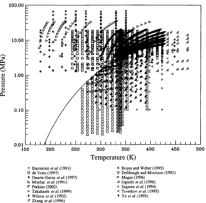
plots, and the comparisons to the equation of state of Sunaga
et al. 共solid lines in the plots兲 are given at this temperature.
Below 270 K, the equation of state represents the data of
Magee 共1996兲, Duarte-Garza et al. 共1997兲, and de Vries
共1997兲 with deviations in density generally less than 0.05%.
Between 270 and 330 K in the liquid, density deviations are
slightly higher for the data of Duarte-Garza et al. and Per-
kins 共2002兲, and somewhat lower 共0.02%兲 for the data of de
Vries and for Defibaugh and Morrison 共1992兲. In the vapor
phase up to 330 K, the datasets are not as consistent as are
those in the liquid, and density deviations tend to be higher,
except for the data of de Vries, which is represented by an
AAD of 0.018%. Deviations for other datasets in this region
are 0.12% for Zhang et al. 共1996兲, 0.08% for Boyes and
Weber 共1995兲, and 0.17% for Ye et al. 共1995兲. Omitting the
data in the region between 3 and 7 mol/dm
3
and at tempera-
tures up to 360 K 共i.e., the critical region兲, the spread in the
data at higher temperatures continues to increase, and the
deviations remain under 0.1% for only the datasets of de
Vries, Zhang et al.,Yeet al., Boyes and Weber, Magee, and
Perkins. Of particular interest in this region are the data of
Perkins, with more than 1200 data points spanning pressures
up to 20 MPa and temperatures up to 429 K. Deviations of
density values calculated using the equation of state from
these data are within about 0.04% in this region.
In the critical region omitted above, from 3 to 7 mol/dm
3
with temperatures to 360 K, deviations in density are no
longer a useful comparison since the uncertainty in the de-
pendent variable pressure 共and to a certain degree tempera-
ture兲 becomes the dominant contribution to the total uncer-
tainty in density. Comparisons of calculated values with even
the most accurate data show average deviations of 0.4% 共de
Vries兲 and 0.85% 共Perkins兲 with maximum errors exceeding
5% in density. In order to compare the equation of state with
experimental data in this region, deviations in pressure are
more meaningful, and the following discussion uses such
deviations as a basis for the discussion of the accuracy of the
representation of experimental values by the equation of
state where the slopes of the isotherms on p–
coordinates
are essentially flat. Figure 24 compares values from the equa-
tion to data in a limited region around the critical point. Most
of the data in this region are represented with average devia-
tions of 0.1%. The scatter in the data is similar for most of
the datasets with deviations of calculated values from the
data of de Vries of about 0.06%. Average deviations for com-
parisons with other datasets are 0.19% for Perkins, 0.27% for
Sagawa et al. 共1994兲, and 0.31% for Defibaugh and Morri-
FIG. 21. Experimental p
T data.
9292 E. W. LEMMON AND R. T JACOBSEN
J. Phys. Chem. Ref. Data, Vol. 34, No. 1, 2005

son. The maximum deviation from the data of de Vries is
0.22%.
Table 8 summarizes the sources for the second virial co-
efficients of R-125. Additional values for the second virial
coefficient were numerically determined by fitting (Z–1)/
as a function of density using the data of de Vries 共1997兲.
The additional data 共values at zero density兲 are shown in Fig.
25 as circles. These values are given in Table 9. Data below
0.1 mol/dm
3
were not used because such low density data
may be subject to larger errors due to local adsorption onto
the walls of the apparatus or to higher uncertainties in the
measurement of extremely low pressures. Additional infor-
mation about the high uncertainties in the second virial co-
efficients at low temperatures was reported by Wagner and
Pruß 共2002兲. The solid lines show isotherms calculated from
the equation of state presented here and the solid curve rep-
resents the saturated vapor density. The y intercept 共zero
density兲 represents the second virial coefficient at a given
temperature, and the third virial coefficient can be taken
from the slope of each line at zero density. The values of the
second virial coefficient calculated from the equation of state
agree well with those determined numerically and shown as
circles in the figure. Comparisons of second virial coeffi-
cients calculated with the equation of state and those deter-
mined from the data of de Vries 共given in Table 9兲 are shown
in Fig. 26. The uncertainty in the derived values at lower
temperatures is higher due to the limited data at densities
above 0.1 mol/dm
3
and to the higher curvature in the data.
5.3. Caloric Data
The sources of experimental data for the speed of sound of
R-125 are summarized in Table 10 and shown graphically in
Fig. 27. Comparisons of values calculated from the equation
of state for the speed of sound are shown in Fig. 28 for the
vapor phase and in Fig. 29 for the liquid phase. The equation
represents the vapor phase data of Gillis 共1997兲 and Ichikawa
et al. 共1998兲 within 0.01% and the liquid phase data of
Takagi 共1996兲 within 0.7%. There are no speed of sound data
below 240 K; however, the extrapolation behavior of the
equation of state is quite reasonable at low temperatures, as
discussed below.
The reported measurements of the isochoric heat capacity,
saturation liquid heat capacity, and isobaric heat capacity
for R-125 are summarized in Table 11 and illustrated in
Fig. 27. Comparisons of values calculated from the equation
of state are shown for the isochoric heat capacities in Fig.
30, saturation liquid heat capacities in Fig. 31, and isobaric
FIG. 22. Experimental p
T data in the critical region.
9393EQUATION OF STATE FOR HFC-125
J. Phys. Chem. Ref. Data, Vol. 34, No. 1, 2005

heat capacities in Fig. 32. Lu
¨
ddecke and Magee 共1996兲
measured both the isochoric heat capacity of R-125 and the
heat capacity along the saturated liquid line. The average
deviation between values from the equation of state and
these data is 0.57% for the isochoric heat capacity and 0.24%
for the saturation liquid heat capacity. There are few experi-
mental data for the isobaric heat capacity of R-125, espe-
cially in the vapor phase 共five points by Wilson et al., 1992兲,
and the data in the liquid phase are not consistent. Although
none of these data were used in the fit, the equation of state
represents the data of Gunther and Steimle 共1997兲 within
0.5%. This agreement indicates consistency between the fit-
ted isochoric and saturation heat capacity data of Lu
¨
ddecke
and Magee and the isobaric heat capacity data of Gunther
and Steimle.
5.4. Extrapolation Behavior
Plots of constant property lines on various thermodynamic
coordinates are useful in assessing the behavior of the equa-
tion of state. The equation developed here was used to pro-
duce plots of temperature versus isochoric heat capacity 共Fig.
FIG. 23. Comparisons of densities calculated with the equation of state to experimental data.
9494 E. W. LEMMON AND R. T JACOBSEN
J. Phys. Chem. Ref. Data, Vol. 34, No. 1, 2005

33兲, isobaric heat capacity 共Fig. 34兲, and speed of sound
共Fig. 35兲. These plots indicate that the equation of state ex-
hibits reasonable behavior over all temperatures and pres-
sures within the range of validity, and that the extrapolation
behavior is reasonable at higher temperatures and pressures.
Additional information about the extrapolation behavior was
given earlier.
6. Estimated Uncertainties of Calculated
Properties
The new reference equation of state for R-125 describes
the p
T surface with an uncertainty (k⫽2) of 0.1% in den-
sity at temperatures from the triple point to 400 K at pres-
sures up to 60 MPa, except in the critical region, where an
uncertainty of 0.2% in pressure is generally attained. In the
limited region between 340 and 400 K and at pressures from
4 to 10 MPa, as well as for all states above 400 K, the
uncertainty in density increases to 0.5%. At temperatures be-
low 330 K and pressures below 30 MPa, the uncertainty in
density in the liquid phase may be as low as 0.04%. In the
vapor and supercritical region, speed of sound data are rep-
resented within 0.05% at pressures below 1 MPa. The esti-
mated uncertainty for heat capacities is 0.5% and the esti-
mated uncertainty for the speed of sound in the liquid phase
FIG. 23. 共Continued.兲
9595EQUATION OF STATE FOR HFC-125
J. Phys. Chem. Ref. Data, Vol. 34, No. 1, 2005

is 0.5% for T⬎ 250 K. The saturation values can be calcu-
lated from the equation of state by application of the Max-
well criterion, which requires equal Gibbs energies and equal
pressures for saturated liquid and vapor states at the same
temperature. The estimated uncertainties of vapor pressures
and saturated liquid densities calculated using the Maxwell
criterion are 0.1% for each property, and the estimated un-
certainty for saturated vapor densities is 0.2%. The uncer-
tainty in density increases as the critical point is approached,
while the accompanying uncertainty in calculated pressures
is 0.2%. As an aid for computer implementation, calculated
values of properties from the equation of state for R-125 are
given in Table 12. The number of digits displayed does not
indicate the accuracy in the values but is given for validation
of computer code.
FIG. 24. Comparisons of pressures calculated with the equation of state to experimental data in the critical region.
TABLE 8. Summary of second virial coefficients
Author
No. of
points
Temp.
range 共K兲
AAD
a
(cm
3
/mol)
Bignell and Dunlop 共1993兲 3 290–310 1.01
Boyes and Weber 共1995兲 8 280–350 2.34
de Vries 共1997兲
b
19 263–413 1.44
Di Nicola et al. 共2002兲 10 303–363 1.23
Gillis 共1997兲 9 240–400 1.91
Grigiante et al. 共2000兲 7 260–360 0.93
Ye et al. 共1995兲 11 290–390 6.40
Zhang et al. 共1995兲 11 290–390 2.60
a
Average absolute difference in the second virial coefficient (cm
3
/mol).
b
Data were derived from the p
T data of de Vries and are given in Table 9.
9696 E. W. LEMMON AND R. T JACOBSEN
J. Phys. Chem. Ref. Data, Vol. 34, No. 1, 2005

7. Acknowledgments
This work was funded by the 21-CR research program of
the Air-Conditioning and Refrigeration Technology Institute;
the Office of Building Technology, State and Community
Programs of the U.S. Department of Energy. We thank Dr.
Mark McLinden of NIST, Boulder, for his assistance and
suggestions during the development and documentation of
the equation. We are also grateful to Dr. Roland Span whose
insights and collaborations have inspired us in various
projects, including this one, over many years.
FIG. 25. Derivation of second virial coefficients from the p
T data of de Vries 共1997兲.
FIG. 26. Comparisons of second virial coefficients calculated with the equation of state to experimental data.
TABLE 9. Second virial coefficients derived from the p
T data of de Vries
共1997兲
Temp. 共K兲 B (dm
3
/mol) Temp. 共K兲 B (dm
3
/mol)
263.150 ⫺ 0.4984 339.152 ⫺ 0.2677
273.150 ⫺ 0.4560 340.150 ⫺ 0.2672
283.151 ⫺ 0.4180 341.153 ⫺ 0.2648
293.151 ⫺ 0.3850 343.152 ⫺ 0.2603
303.150 ⫺ 0.3529 346.152 ⫺ 0.2548
313.150 ⫺ 0.3269 353.150 ⫺ 0.2426
323.150 ⫺ 0.3028 363.152 ⫺ 0.2254
333.150 ⫺ 0.2808 373.152 ⫺ 0.2095
335.150 ⫺ 0.2766 393.150 ⫺ 0.1837
337.151 ⫺ 0.2722 413.152 ⫺ 0.1603
9797EQUATION OF STATE FOR HFC-125
J. Phys. Chem. Ref. Data, Vol. 34, No. 1, 2005
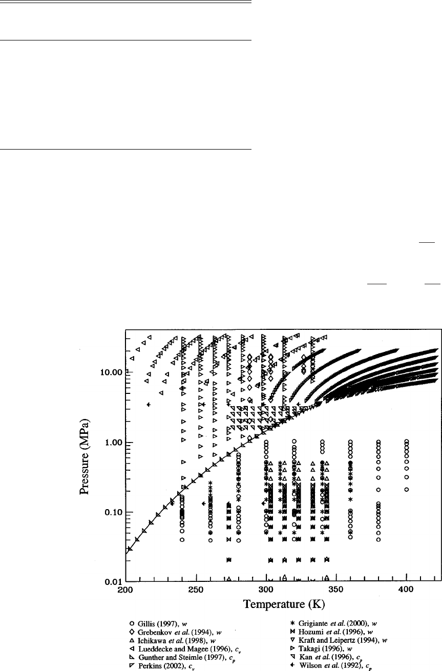
8. Appendix A: Thermodynamic Equations
The functional form of the Helmholtz energy equation of
state is explicit in the dimensionless Helmholtz energy,
␣
,
using independent variables of dimensionless density and
temperature,
␣
共
␦
,
兲
⫽
␣
0
共
␦
,
兲
⫹
␣
r
共
␦
,
兲
, 共40兲
where
␦
⫽
/
c
and
⫽ T
c
/T. The ideal gas Helmholtz en-
ergy is
␣
0
⫽ ln
␦
⫺ ln
⫹
兺
k⫽ 1
3
a
k
t
k
⫹
兺
k⫽ 4
6
a
k
ln
关
1⫺ exp
共
⫺ b
k
兲
兴
,
共41兲
and the residual fluid Helmholtz energy is
␣
r
共
␦
,
兲
⫽
兺
k⫽ 1
5
N
k
␦
d
k
t
k
⫹
兺
k⫽ 6
15
N
k
␦
d
k
t
k
exp
共
⫺
␦
l
k
兲
⫹
兺
k⫽ 16
18
N
k
␦
d
k
t
k
exp
共
⫺
␦
l
k
兲
exp
共
⫺
m
k
兲
.
共42兲
The functions used for calculating pressure (p), compress-
ibility factor (Z), internal energy (u), enthalpy (h), entropy
(s), Gibbs energy (g), isochoric heat capacity (c
), isobaric
heat capacity (c
p
), and the speed of sound (w) from Eq. 共3兲
are given below.
p⫽
RT
冋
1⫹
␦
冉
␣
r
␦
冊
册
共43兲
Z⫽
p
RT
⫽ 1⫹
␦
冉
␣
r
␦
冊
共44兲
FIG. 27. Experimental isobaric and isochoric heat capacities and speed of sound data.
TABLE 10. Summary of speed of sound data
Author
No. of
points
Temp.
range
共K兲
Pressure
range
共MPa兲
AAD
共%兲
Vapor Phase Data
Hozumi et al. 共1996兲 72 273–343 0.01–0.24 0.034
Ichikawa et al. 共1998兲 74 273–343 0.01–0.50 0.007
Grigiante et al. 共2000兲 69 260–360 0.05–0.50 0.019
Gillis 共1997兲 149 240–400 0.04–1.02 0.008
Liquid Phase and Saturation Data
Grebenkov et al. 共1994兲 30 288–333 1.14–16.4 0.233
Kraft and Leipertz 共1994兲 13 293–338 Sat. liq. 2.211
Kraft and Leipertz 共1994兲 9 307–338 Sat. vap. 1.560
Takagi 共1996兲 167 241–333 0.23–32.2 0.264
9898 E. W. LEMMON AND R. T JACOBSEN
J. Phys. Chem. Ref. Data, Vol. 34, No. 1, 2005

u
RT
⫽
冋
冉
␣
0
冊
␦
⫹
冉
␣
r
冊
␦
册
共45兲
h
RT
⫽
冋
冉
␣
0
冊
␦
⫹
冉
␣
r
冊
␦
册
⫹
␦
冉
␣
r
␦
冊
⫹ 1 共46兲
s
R
⫽
冋
冉
␣
0
冊
␦
⫹
冉
␣
r
冊
␦
册
⫺
␣
0
⫺
␣
r
共47兲
g
RT
⫽ 1⫹
␣
0
⫹
␣
r
⫹
␦
冉
␣
r
␦
冊
共48兲
c
R
⫽⫺
2
冋
冉
2
␣
0
2
冊
␦
⫹
冉
2
␣
r
2
冊
␦
册
共49兲
c
p
R
⫽
c
R
⫹
冋
1⫹
␦
冉
␣
r
␦
冊
⫺
␦
冉
2
␣
r
␦
冊
册
2
冋
1⫹ 2
␦
冉
␣
r
␦
冊
⫹
␦
2
冉
2
␣
r
␦
2
冊
册
共50兲
w
2
M
RT
⫽ 1⫹2
␦
冉
␣
r
␦
冊
⫹
␦
2
冉
2
␣
r
␦
2
冊
⫺
冋
1⫹
␦
冉
␣
r
␦
冊
⫺
␦
冉
2
␣
r
␦
冊
册
2
2
冋
冉
2
␣
0
2
冊
␦
⫹
冉
2
␣
r
2
冊
␦
册
共51兲
The fugacity coefficient and second and third virial coeffi-
cients are given by Eqs. 共52兲–共54兲.
⫽ exp
关
Z⫺ 1⫺ ln
共
Z
兲
⫹
␣
r
兴
共52兲
B
共
T
兲
⫽ lim
␦
→ 0
冋
1
c
冉
␣
r
␦
冊
册
共53兲
C
共
T
兲
⫽ lim
␦
→ 0
冋
1
c
2
冉
2
␣
r
␦
2
冊
册
共54兲
Other derived properties, given in Eqs. 共55兲–共57兲, include
the first derivative of pressure with respect to density at con-
stant temperature (
p/
)
T
, the second derivative of pres-
sure with respect to density at constant temperature
FIG. 28. Comparisons of speeds of sound in the vapor phase calculated with the equation of state to experimental data.
9999EQUATION OF STATE FOR HFC-125
J. Phys. Chem. Ref. Data, Vol. 34, No. 1, 2005

(
2
p/
2
)
T
, and the first derivative of pressure with respect
to temperature at constant density (
p/
T)
.
冉
p
冊
T
⫽ RT
冋
1⫹ 2
␦
冉
␣
r
␦
冊
⫹
␦
2
冉
2
␣
r
␦
2
冊
册
共55兲
冉
2
p
2
冊
T
⫽
RT
冋
2
␦
冉
␣
r
␦
冊
⫹ 4
␦
2
冉
2
␣
r
␦
2
冊
⫹
␦
3
冉
3
␣
r
␦
3
冊
册
共56兲
冉
p
T
冊
⫽ R
冋
1⫹
␦
冉
␣
r
␦
冊
⫺
␦
冉
2
␣
r
␦
冊
册
共57兲
Equations for additional thermodynamic properties such as
the isothermal compressibility and the Joule–Thomson coef-
ficient are given in Lemmon et al. 共2000兲.
The derivatives of the ideal gas Helmholtz energy required
by the equations for the thermodynamic properties are
FIG. 29. Comparisons of speeds of sound in the liquid phase calculated with the equation of state to experimental data.
TABLE 11. Summary of experimental heat capacity data
Author
No. of
points
Temp.
range
共K兲
Density
range
(mol/dm
3
)
Pressure
range
共MPa兲
AAD
共%兲
Isochoric Heat Capacity Data
Perkins 共2002兲 474 305–397 4.00–19.5 1.185
Lu
¨
ddecke and Magee 共1996兲 99 200–342 10.5–13.5 0.577
Saturation Heat Capacity Data
Lu
¨
ddecke and Magee 共1996兲 93 176–278 0.244
Isobaric Heat Capacity Data
Kan et al. 共1996兲 78 276–328 1.59–3.04 1.820
Wilson et al. 共1992兲 10 216–333 0.13–3.45 1.182
Gunther and Steimle 共1997兲 24 203–318 Sat. liq. 0.520
100100 E. W. LEMMON AND R. T JACOBSEN
J. Phys. Chem. Ref. Data, Vol. 34, No. 1, 2005

FIG. 30. Comparisons of isochoric heat capacities calculated with the equation of state to experimental data.
FIG. 31. Comparisons of saturation heat capacities calculated with the equation of state to experimental data.
101101EQUATION OF STATE FOR HFC-125
J. Phys. Chem. Ref. Data, Vol. 34, No. 1, 2005

␣
0
⫽⫺1⫹
兺
k⫽ 1
3
t
k
a
k
t
k
⫹
兺
k⫽ 4
6
a
k
b
k
冋
1
exp
共
b
k
兲
⫺ 1
册
,
共58兲
and
2
2
␣
0
2
⫽ 1⫹
兺
k⫽ 1
3
t
k
共
t
k
⫺ 1
兲
a
k
t
k
⫺
2
兺
k⫽ 4
6
a
k
b
k
2
exp
共
b
k
兲
关
exp
共
b
k
兲
⫺ 1
兴
2
. 共59兲
The derivatives of the residual Helmholtz energy are given in
Eqs. 共60兲–共65兲.
␦
␣
r
␦
⫽
兺
k⫽ 1
5
d
k
N
k
␦
d
k
t
k
⫹
兺
k⫽ 6
15
N
k
␦
d
k
t
k
exp
共
⫺
␦
l
k
兲
⫻
共
d
k
⫺ l
k
␦
l
k
兲
⫹
兺
k⫽ 16
18
N
k
␦
d
k
t
k
exp
共
⫺
␦
l
k
兲
⫻ exp
共
⫺
m
k
兲
共
d
k
⫺ l
k
␦
l
k
兲
共60兲
FIG. 32. Comparisons of isobaric heat capacities calculated with the equation of state to experimental data.
FIG. 33. Isochoric heat capacity versus temperature diagram.
102102 E. W. LEMMON AND R. T JACOBSEN
J. Phys. Chem. Ref. Data, Vol. 34, No. 1, 2005

FIG. 34. Isobaric heat capacity versus temperature diagram.
FIG. 35. Speed of sound versus temperature diagram.
103103EQUATION OF STATE FOR HFC-125
J. Phys. Chem. Ref. Data, Vol. 34, No. 1, 2005

␦
2
2
␣
r
␦
2
⫽
兺
k⫽ 1
5
d
k
共
d
k
⫺ 1
兲
N
k
␦
d
k
t
k
⫹
兺
k⫽ 6
15
N
k
␦
d
k
t
k
exp
共
⫺
␦
l
k
兲
⫻
关共
d
k
⫺ l
k
␦
l
k
兲
共
d
k
⫺ 1⫺ l
k
␦
l
k
兲
⫺ l
k
2
␦
l
k
兴
⫹
兺
k⫽ 16
18
N
k
␦
d
k
t
k
exp
共
⫺
␦
l
k
兲
exp
共
⫺
m
k
兲
⫻
关共
d
k
⫺ l
k
␦
l
k
兲
共
d
k
⫺ 1⫺ l
k
␦
l
k
兲
⫺ l
k
2
␦
l
k
兴
共61兲
␦
3
3
␣
r
␦
3
⫽
兺
k⫽ 1
5
d
k
共
d
k
⫺ 1
兲
共
d
k
⫺ 2
兲
N
k
␦
d
k
t
k
⫹
兺
k⫽ 6
15
N
k
␦
d
k
t
k
exp
共
⫺
␦
l
k
兲
兵
d
k
共
d
k
⫺ 1
兲
共
d
k
⫺ 2
兲
⫹
␦
l
k
关
⫺ 2l
k
⫹ 6d
k
l
k
⫺ 3d
k
2
l
k
⫺ 3d
k
l
k
2
⫹ 3l
k
2
⫺ l
k
3
兴
⫹
␦
2l
k
关
3d
k
l
k
2
⫺ 3l
k
2
⫹ 3l
k
3
兴
⫺ l
k
3
␦
3l
k
其
⫹
兺
k⫽ 16
18
N
k
␦
d
k
t
k
exp
共
⫺
␦
l
k
兲
exp
共
⫺
m
k
兲
⫻
兵
d
k
共
d
k
⫺ 1
兲
共
d
k
⫺ 2
兲
⫹
␦
l
k
关
⫺ 2l
k
⫹ 6d
k
l
k
⫺ 3d
k
2
l
k
⫺ 3d
k
l
k
2
⫹ 3l
k
2
⫺ l
k
3
兴
⫹
␦
2l
k
关
3d
k
l
k
2
⫺ 3l
k
2
⫹ 3l
k
3
兴
⫺ l
k
3
␦
3l
k
其
共62兲
␣
r
⫽
兺
k⫽ 1
5
t
k
N
k
␦
d
k
t
k
⫹
兺
k⫽ 6
15
t
k
N
k
␦
d
k
t
k
exp
共
⫺
␦
l
k
兲
⫹
兺
k⫽ 16
18
N
k
␦
d
k
t
k
exp
共
⫺
␦
l
k
兲
exp
共
⫺
m
k
兲
⫻
共
t
k
⫺ m
k
m
k
兲
共63兲
2
2
␣
r
2
⫽
兺
k⫽ 1
5
t
k
共
t
k
⫺ 1
兲
N
k
␦
d
k
t
k
⫹
兺
k⫽ 6
15
t
k
共
t
k
⫺ 1
兲
N
k
␦
d
k
t
k
⫻ exp
共
⫺
␦
l
k
兲
⫹
兺
k⫽ 16
18
N
k
␦
d
k
t
k
exp
共
⫺
␦
l
k
兲
⫻ exp
共
⫺
m
k
兲
关共
t
k
⫺ m
k
m
k
兲
共
t
k
⫺ 1⫺ m
k
m
k
兲
⫺ m
k
2
m
k
兴
共64兲
␦
2
␣
r
␦
⫽
兺
k⫽ 1
5
d
k
t
k
N
k
␦
d
k
t
k
⫹
兺
k⫽ 6
15
t
k
N
k
␦
d
k
t
k
exp
共
⫺
␦
l
k
兲
⫻
共
d
k
⫺ l
k
␦
l
k
兲
⫹
兺
k⫽ 16
18
N
k
␦
d
k
t
k
exp
共
⫺
␦
l
k
兲
⫻ exp
共
⫺
m
k
兲
共
d
k
⫺ l
k
␦
l
k
兲
共
t
k
⫺ m
k
m
k
兲
共65兲
9. Appendix B: Tables of Thermodynamic Properties of R-125 at Saturation
T
(°C)
p
共MPa兲
(kg/m
3
)
h
共kJ/kg兲
s
共kJ/共kg K兲兲
c
v
共kJ/共kg K兲兲
c
p
共kJ/共kg K兲兲
w
共m/s兲
⫺ 100.630 0.002 91 1690.7 87.130 .490 22 0.6776 1.035 932.6
0.244 62 277.39 1.5931 0.4984 0.5689 116.4
⫺ 100. 0.003 09 1688.7 87.782 .493 99 0.6781 1.035 929.2
0.258 34 277.74 1.5911 0.4997 0.5703 116.6
⫺ 95. 0.004 81 1672.5 92.969 .523 52 0.6818 1.040 903.2
0.391 79 280.54 1.5764 0.5099 0.5810 118.0
⫺ 90. 0.007 29 1656.2 98.181 .552 36 0.6860 1.045 877.5
0.577 94 283.36 1.5634 0.5201 0.5919 119.4
⫺ 85. 0.010 74 1639.9 103.42 .58059 0.6906 1.051 852.3
0.831 42 286.20 1.5520 0.5304 0.6031 120.7
⫺ 80. 0.015 47 1623.4 108.70 .60824 0.6955 1.058 827.5
1.1691 289.06 1.5421 0.5409 0.6146 121.9
TABLE 12. Calculated values of properties for algorithm verification
Temperature
共K兲
Density
(mol/dm
3
)
Pressure
共MPa兲
Isochoric heat
capacity
(J/mol•K)
Isobaric heat
capacity
(J/mol•K)
Speed of
sound
共m/s兲
200.0 14.0 42.302 520 85.816 305 123.536 41 968.671 94
300.0 10.0 2.902 3498 99.919 660 164.169 14 345.912 35
300.0 0.7 1.324 5058 94.823 171 124.960 09 120.560 07
400.0 5.0 9.049 5658 114.418 19 198.117 92 151.530 60
339.2 4.8 3.620 1215 130.636 50 274 863.02 78.735 928
104104 E. W. LEMMON AND R. T JACOBSEN
J. Phys. Chem. Ref. Data, Vol. 34, No. 1, 2005

T
(°C兲
p
共MPa兲
(kg/m
3
兲
h
共kJ/kg兲
s
共kJ/共kg K兲兲
c
v
共kJ/共kg K兲兲
c
p
共kJ/共kg K兲兲
w
共m/s兲
⫺ 75. 0.02179 1606.7 114.01 .635 37 0.7006 1.066 802.9
1.6103 291.94 1.5333 0.5514 0.6264 123.1
⫺ 70. 0.03008 1589.9 119.36 .662 01 0.7060 1.074 778.6
2.1766 294.83 1.5257 0.5620 0.6385 124.1
⫺ 65. 0.04076 1572.9 124.75 .688 21 0.7115 1.082 754.5
2.8921 297.71 1.5191 0.5727 0.6511 125.1
⫺ 60. 0.05432 1555.7 130.19 .713 98 0.7171 1.091 730.6
3.7833 300.60 1.5135 0.5836 0.6641 126.0
⫺ 55. 0.07126 1538.2 135.68 .739 37 0.7229 1.101 706.8
4.8791 303.48 1.5086 0.5946 0.6776 126.8
⫺ 50. 0.09216 1520.5 141.21 .764 39 0.7288 1.111 683.2
6.2112 306.35 1.5044 0.6058 0.6916 127.4
⫺ 45. 0.117 63 1502.4 146.80 .789 07 0.7349 1.121 659.6
7.8140 309.20 1.5009 0.6171 0.7063 127.9
⫺ 40. 0.14830 1484.0 152.44 .813 45 0.7410 1.132 636.1
9.7249 312.03 1.4980 0.6286 0.7216 128.3
⫺ 35. 0.18487 1465.3 158.14 .837 53 0.7473 1.144 612.6
11.985 314.84 1.4955 0.6402 0.7376 128.6
⫺ 30. 0.22806 1446.1 163.90 .861 35 0.7537 1.157 589.1
14.639 317.61 1.4935 0.6520 0.7545 128.7
⫺ 25. 0.27861 1426.5 169.73 .884 93 0.7602 1.170 565.7
17.736 320.34 1.4919 0.6640 0.7724 128.7
⫺ 20. 0.33733 1406.4 175.62 .908 29 0.7668 1.184 542.2
21.331 323.03 1.4906 0.6761 0.7912 128.5
⫺ 15. 0.40501 1385.8 181.59 .931 45 0.7736 1.199 518.7
25.486 325.67 1.4895 0.6882 0.8112 128.1
⫺ 10. 0.48252 1364.5 187.64 .954 43 0.7805 1.216 495.2
30.271 328.24 1.4887 0.7003 0.8324 127.5
⫺ 5. 0.57072 1342.6 193.77 .977 28 0.7876 1.234 471.6
35.768 330.74 1.4881 0.7122 0.8550 126.8
0. 0.670 52 1319.8 200.00 1.0000 0.7948 1.255 448.0
42.070 333.16 1.4875 0.7240 0.8797 125.8
5. 0.782 88 1296.2 206.33 1.0226 0.8021 1.277 424.3
49.291 335.47 1.4869 0.7359 0.9073 124.6
10. 0.908 75 1271.5 212.76 1.0452 0.8095 1.303 400.4
57.564 337.66 1.4863 0.7483 0.9392 123.2
15. 1.049 18 1245.6 219.32 1.0678 0.8172 1.332 376.3
67.054 339.71 1.4856 0.7617 0.9770 121.5
20. 1.205 20 1218.3 226.02 1.0904 0.8252 1.367 352.0
77.966 341.58 1.4846 0.7764 1.023 119.6
25. 1.377 92 1189.4 232.87 1.1131 0.8335 1.407 327.4
90.557 343.26 1.4834 0.7928 1.080 117.3
30. 1.568 53 1158.4 239.91 1.1359 0.8425 1.457 302.4
105.17 344.71 1.4817 0.8111 1.152 114.8
35. 1.778 27 1125.0 247.16 1.1591 0.8522 1.521 276.9
122.27 345.88 1.4794 0.8315 1.245 111.9
40. 2.008 49 1088.4 254.67 1.1826 0.8630 1.605 250.8
142.52 346.69 1.4764 0.8542 1.372 108.6
45. 2.260 74 1047.7 262.52 1.2067 0.8755 1.724 223.8
166.95 347.05 1.4724 0.8796 1.553 104.8
50. 2.536 80 1001.1 270.83 1.2318 0.8907 1.910 195.6
197.29 346.75 1.4667 0.9083 1.842 100.5
55. 2.838 91 945.35 279.83 1.2585 0.9106 2.252 165.3
105105EQUATION OF STATE FOR HFC-125
J. Phys. Chem. Ref. Data, Vol. 34, No. 1, 2005

T
(°C兲
p
共MPa兲
(kg/m
3
兲
h
共kJ/kg兲
s
共kJ/共kg K兲兲
c
v
共kJ/共kg K兲兲
c
p
共kJ/共kg K兲兲
w
共m/s兲
236.92 345.44 1.4584 0.9421 2.386 95.6
60. 3.170 28 872.09 290.10 1.2884 0.9411 3.139 131.5
294.37 342.21 1.4448 0.9856 3.833 89.8
65. 3.536 97 735.11 304.88 1.3311 1.014 13.67 90.0
416.57 332.24 1.4120 1.060 20.07 82.6
66. 3.616 07 612.97 314.86 1.3602 1.078 818.2 78.9
534.59 321.41 1.3795 1.093 923.0 79.2
66.023 3.617 70 573.58 318.06 1.3696
⫺ 100.630 0.002 91 1690.7 87.130 .490 22 0.6776 1.035 932.6
0.244 62 277.39 1.5931 0.4984 0.5689 116.4
⫺ 76.278 0.02 1611.0 112.65 .628 49 0.6993 1.064 809.2
1.4866 291.20 1.5355 0.5487 0.6233 122.8
⫺ 65.319 0.04 1574.0 124.41 .686 55 0.7111 1.082 756.1
2.8415 297.53 1.5195 0.5721 0.6503 125.0
⫺ 58.200 0.06 1549.4 132.16 .723 16 0.7192 1.095 722.0
4.1526 301.64 1.5116 0.5876 0.6689 126.3
⫺ 52.785 0.08 1530.4 138.12 .750 49 0.7255 1.105 696.3
5.4381 304.75 1.5067 0.5996 0.6837 127.1
⫺ 48.356 0.10 1514.6 143.04 .772 54 0.7308 1.114 675.4
6.7064 307.29 1.5032 0.6095 0.6964 127.6
⫺ 48.089 0.101 325 1513.6 143.34 .773 86 0.7311 1.115 674.2
6.7900 307.44 1.5030 0.6101 0.6971 127.6
⫺ 39.747 0.15 1483.1 152.73 .814 67 0.7413 1.133 634.9
9.8304 312.18 1.4978 0.6292 0.7224 128.4
⫺ 33.154 0.20 1458.3 160.26 .846 35 0.7496 1.149 603.9
12.916 315.87 1.4947 0.6446 0.7438 128.7
⫺ 27.735 0.25 1437.3 166.53 .872 06 0.7566 1.162 578.5
15.984 318.85 1.4927 0.6574 0.7625 128.7
⫺ 23.093 0.30 1418.9 171.97 .893 86 0.7627 1.175 556.7
19.045 321.37 1.4913 0.6686 0.7795 128.6
⫺ 19.009 0.35 1402.4 176.80 .912 89 0.7681 1.187 537.6
22.108 323.56 1.4904 0.6785 0.7951 128.4
⫺ 15.347 0.40 1387.3 181.18 .929 84 0.7731 1.198 520.4
25.178 325.49 1.4896 0.6874 0.8098 128.1
⫺ 12.018 0.45 1373.2 185.19 .945 18 0.7777 1.209 504.7
28.259 327.21 1.4890 0.6954 0.8237 127.8
⫺ 8.957 0.50 1360.0 188.91 .959 21 0.7820 1.220 490.3
31.356 328.77 1.4886 0.7028 0.8370 127.4
⫺ 6.119 0.55 1347.6 192.39 .972 17 0.7860 1.230 476.9
34.471 330.19 1.4882 0.7095 0.8498 127.0
⫺ 3.469 0.60 1335.7 195.67 .984 24 0.7898 1.240 464.4
37.607 331.49 1.4879 0.7158 0.8623 126.5
⫺ 0.980 0.65 1324.3 198.77 .995 55 0.7933 1.251 452.6
40.766 332.69 1.4876 0.7217 0.8747 126.0
1.369 0.70 1313.4 201.72 1.0062 0.7967 1.261 441.5
43.951 333.80 1.4873 0.7272 0.8869 125.5
3.596 0.75 1302.9 204.54 1.0163 0.8000 1.271 431.0
47.163 334.83 1.4871 0.7325 0.8992 125.0
5.714 0.80 1292.7 207.24 1.0259 0.8031 1.281 420.9
50.404 335.79 1.4869 0.7377 0.9116 124.4
7.735 0.85 1282.8 209.83 1.0350 0.8061 1.291 411.2
53.677 336.68 1.4866 0.7426 0.9242 123.8
106106 E. W. LEMMON AND R. T JACOBSEN
J. Phys. Chem. Ref. Data, Vol. 34, No. 1, 2005

T
(°C兲
p
共MPa兲
(kg/m
3
兲
h
共kJ/kg兲
s
共kJ/共kg K兲兲
c
v
共kJ/共kg K兲兲
c
p
共kJ/共kg K兲兲
w
共m/s兲
9.670 0.90 1273.1 212.33 1.0437 0.8090 1.301 402.0
56.982 337.52 1.4864 0.7475 0.9370 123.3
11.525 0.95 1263.7 214.75 1.0521 0.8118 1.311 393.1
60.321 338.30 1.4861 0.7523 0.9500 122.7
13.309 1.00 1254.5 217.09 1.0602 0.8146 1.322 384.5
63.697 339.03 1.4858 0.7570 0.9635 122.1
16.686 1.10 1236.6 221.56 1.0754 0.8198 1.343 368.1
70.564 340.36 1.4853 0.7665 0.9915 120.9
19.841 1.20 1219.2 225.80 1.0897 0.8249 1.365 352.8
77.596 341.53 1.4847 0.7759 1.021 119.6
22.806 1.30 1202.3 229.84 1.1031 0.8298 1.389 338.2
84.806 342.55 1.4839 0.7854 1.053 118.3
25.605 1.40 1185.7 233.71 1.1158 0.8346 1.413 324.4
92.209 343.45 1.4832 0.7949 1.088 117.0
28.258 1.50 1169.4 237.43 1.1280 0.8393 1.439 311.1
99.823 344.24 1.4823 0.8045 1.125 115.7
30.781 1.60 1153.4 241.02 1.1395 0.8439 1.466 298.4
107.66 344.91 1.4814 0.8141 1.165 114.3
33.189 1.70 1137.4 244.50 1.1507 0.8486 1.496 286.2
115.75 345.49 1.4803 0.8238 1.208 113.0
35.492 1.80 1121.5 247.88 1.1614 0.8532 1.528 274.3
124.11 345.98 1.4792 0.8336 1.256 111.6
39.823 2.00 1089.8 254.40 1.1817 0.8626 1.602 251.7
141.74 346.67 1.4766 0.8534 1.366 108.7
43.837 2.20 1057.6 260.66 1.2010 0.8724 1.692 230.2
160.82 347.01 1.4734 0.8734 1.504 105.7
47.578 2.40 1024.5 266.74 1.2195 0.8829 1.809 209.4
181.71 346.99 1.4697 0.8939 1.684 102.7
51.084 2.60 989.96 272.71 1.2374 0.8945 1.966 189.2
204.93 346.57 1.4652 0.9151 1.930 99.5
54.381 2.80 952.95 278.66 1.2550 0.9077 2.194 169.2
231.31 345.68 1.4596 0.9375 2.294 96.2
57.490 3.00 912.04 284.72 1.2728 0.9237 2.565 149.1
262.29 344.18 1.4526 0.9620 2.893 92.8
60.426 3.20 864.39 291.08 1.2912 0.9446 3.288 128.4
300.75 341.78 1.4432 0.9901 4.077 89.3
63.198 3.40 802.42 298.28 1.3120 0.9757 5.402 106.5
354.37 337.68 1.4292 1.02 7.502 85.6
65.800 3.60 668.27 310.49 1.3474 1.052 71.10 81.4
480.94 326.28 1.3940 1.085 95.87 80.5
66.023 3.6177 573.58 318.06 1.3696
10. References
Angus, S., B. Armstrong, and K. M. de Reuck, International Thermody-
namic Tables of the Fluid State-7 Propylene, International Union of
Pure and Applied Chemistry 共Pergamon Press, Oxford, 1980兲.
Baroncini, C., G. Giuliani, and F. Polonara, 3rd World Conf. on Experimen-
tal Heat Transfer, Fluid Mechanics and Thermodynamics, Vol. 2, 1993,
p. 1774.
Bignell, C. M. and P. J. Dunlop, J. Chem. Phys. 98, 4889 共1993兲.
Boyes, S. J. and L. A. Weber, J. Chem. Thermodyn. 27,163共1995兲.
Bu
¨
cker, D. and W. Wagner, J. Phys. Chem. Ref. Data 共in press, 2004兲.
Chen, S. S., A. S. Rodgers, J. Chao, R. C. Wilhoit, and B. J. Zwolinski, J.
Phys. Chem. Ref. Data 4,441共1975兲.
Defibaugh, D. R. and G. Morrison, Fluid Phase Equilib. 80,157共1992兲.
Deiters, U. K. and K. M. de Reuck, Pure Appl. Chem. 69, 1237 共1997兲.
de Reuck, K. M., International Thermodynamic Tables of the Fluid State-11
Fluorine, International Union of Pure and Applied Chemistry 共Perga-
mon Press, Oxford, 1990兲.
de Reuck, K. M. and R. J. B. Craven, International Thermodynamic Tables
of the Fluid State-12 Methanol, International Union of Pure and Applied
Chemistry 共Blackwell Scientific Publications, London, 1993兲.
de Reuck, K. M., R. J. B. Craven, and W. A. Cole, Report on the Develop-
ment of an Equation of State for Sulphur Hexafluoride, IUPAC Thermo-
dynamic Tables Project Centre, London, 1991.
de Vries, B., Thermodynamische Eigenschaften der Alternativen Kauelte-
mittel R32, R125 und R143a—Messungen und Zustandsgleichungen,
Dissertation, University of Hannover, Germany, 1997.
107107EQUATION OF STATE FOR HFC-125
J. Phys. Chem. Ref. Data, Vol. 34, No. 1, 2005
de Vries, B., R. Tillner-Roth, and H. D. Baehr, 19th International Congress
of Refrigeration, The Hague, The Netherlands, International Institute of
Refrigeration, Vol. IVa, 1995, p. 582.
Di Nicola, G., G. Giuliani, F. Polonara, R. Stryjek, Fluid Phase Equilib. 199,
161 共2002兲.
Duarte-Garza, H. A. and J. W. Magee, Int. J. Thermophys. 18, 173 共1997兲.
Duarte-Garza, H. A., C. E. Stouffer, K. R. Hall, J. C. Holste, K. N. Marsh,
and B. E. Gammon, J. Chem. Eng. Data 42,745共1997兲.
Elhassan, A. E., R. J. B. Craven, and K. M. de Reuck, Fluid Phase Equilib.
130,167共1997兲.
Ely, J. F., Colorado School of Mines, Golden, Colorado 共private communi-
cation, 1995兲.
Fukushima, M. and S. Ohotoshi, 13th Japan Symp. Thermophys. Prop.,
1992, p. 49.
Gillis, K. A., Int. J. Thermophys. 18,73共1997兲.
Gorenflo, D., R. Koester, and G. Herres, Universita
¨
t Paderborn, Germany
共private communication, 1996兲.
Grebenkov, A. J., Yu. G. Kotelevsky, V. V. Saplitza, O. V. Beljaeva, T. A.
Zajatz, and B. D. Timofeev, Proc. CFC’s: The Day After, IIR Comm B1,
B2, E1, E2, 1994, p. 21.
Grigiante, M., G. Scalabrin, G. Benedetto, R. M. Gavioso, and R. Spagnolo,
Fluid Phase Equilib. 174,69共2000兲.
Gunther, D. and F. Steimle, Int. J. Refrig. 20, 235 共1997兲.
Higashi, Y., Int. J. Refrig. 17, 524 共1994兲.
Holian, K. S., T-1 Handbook of Material Properties Data Bases, Vol. Ic:
Equations of State 共Los Alamos National Laboratory, 1984兲, Report No.
LA-10160-MS.
Hozumi, T., H. Sato, and K. Watanabe, Int. J. Thermophys. 17, 587 共1996兲.
Ichikawa, T., K. Ogawa, H. Sato, and K. Watanabe, Speed-of-Sound Mea-
surements for Gaseous Pentafluoroethane and Binary Mixture of
Pentafluoroethane⫹1,1,1-Trifluoroethane, Department of System Design
Engineering, Faculty of Science and Technology, Keio University, Yoko-
hama, Japan, 1998.
Jacobsen, R. T, S. G. Penoncello, and E. W. Lemmon, Fluid Phase Equilib.
80,45共1992兲.
Kamei, A., S. W. Beyerlein, and R. T Jacobsen, Int. J. Thermophys. 16, 1155
共1995兲.
Kan, T., G. Yasuda, M. Suzuki, H. Sato, and K. Watanabe, Proc. 33rd Na-
tional Heat Transfer Symposium of Japan, Nigata, Japan, 1996, p. 169.
Katti, R. S., R. T Jacobsen, R. B. Stewart, and M. Jahangiri, Adv. Cryo. Eng.
31,1189共1986兲.
Kraft, K. and A. Leipertz, Int. J. Thermophys. 15, 387 共1994兲.
Kuwabara, S., H. Aoyama, H. Sato, and K. Watanabe, J. Chem. Eng. Data
40,112共1995兲.
Lee, B.-G., J.-Y. Park, J. S. Lim, and Y.-W. Lee, J. Chem. Eng. Data 45, 760
共2000兲.
Lemmon, E. W. and R. T Jacobsen, J. Phys. Chem. Ref. Data 29, 521
共2000兲.
Lemmon, E. W., R. T Jacobsen, S. G. Penoncello, and D. G. Friend, J. Phys.
Chem. Ref. Data 29,331共2000兲.
Lu
¨
ddecke, T. O. and J. W. Magee, Int. J. Thermophys. 17,823共1996兲.
Magee, J. W., Int. J. Thermophys. 17, 803 共1996兲.
Marx, V., A. Pruß, and W. Wagner, Fortschr.-Ber. VDI, Dusseldorf: VDI-
Verlag 19共57兲共1992兲.
McCarty, R. D. and V. D. Arp, Adv. Cryo. Eng. 35, 1465 共1990兲.
Miyamoto, H. and K. Watanabe, Int. J. Thermophys. 21,1045共2000兲.
Mohr, P. J. and B. N. Taylor, J. Phys. Chem. Ref. Data 28,1713共1999兲.
Monluc, Y., T. Sagawa, H. Sato, and K. Watanabe, Proc. 12th Japan Symp.
Thermophys. Prop., 1991, p. 65.
Nagel, M. and K. Bier, DKV-Tagungsbericht 20,39共1993兲.
Oguchi, K., A. Murano, K. Omata, and N. Yada, Int. J. Thermophys. 17,55
共1996兲.
Outcalt, S. L. and M. O. McLinden, Int. J. Thermophys. 16,79共1995兲.
Outcalt, S. L. and M. O. McLinden, J. Phys. Chem. Ref. Data 25,605
共1996兲.
Penoncello, S. G., A. R. H. Goodwin, and R. T Jacobsen, Int. J. Thermo-
phys. 16, 519 共1995兲.
Penoncello, S. G., E. W. Lemmon, R. T Jacobsen, and Z. Shan, J. Phys.
Chem. Ref. Data 32, 1473 共2003兲.
Perkins, R. A., NIST, 325 Broadway, Boulder, Colorado 共private communi-
cation, 2002兲.
Piao, C.-C. and M. Noguchi, J. Phys. Chem. Ref. Data 27,775共1998兲.
Preston-Thomas, H., Metrologia 27,3共1990兲.
Sagawa, T., M. S. Thesis, Keio University, 1994.
Sagawa, T., H. Sato, and K. Watanabe, High Temp.-High Press. 26, 193
共1994兲.
Schmidt, J. W. and M. R. Moldover, J. Chem. Eng. Data 39,39共1994兲.
Schmidt, R. and W. Wagner, Fluid Phase Equilib. 19,175共1985兲.
Setzmann, U. and W. Wagner, J. Phys. Chem. Ref. Data 20,1061共1991兲.
Singh, R. R., E. A. E. Lund, and I. R. Shankland, Proc. CFC and Halon
International Conference, 1991, p. 451.
Smukala, J., R. Span, and W. Wagner, J. Phys. Chem. Ref. Data 29, 1053
共2000兲.
Span, R., Multiparameter Equations of State—An Accurate Source of Ther-
modynamic Property Data 共Springer, Berlin, 2000兲.
Span, R., E. W. Lemmon, R. T Jacobsen, W. Wagner, and A. Yokozeki, J.
Phys. Chem. Ref. Data 29,1361共2000兲.
Span, R. and W. Wagner, J. Phys. Chem. Ref. Data 25, 1509 共1996兲.
Span, R. and W. Wagner, Int. J. Thermophys. 18, 1415 共1997兲.
Sunaga, H., R. Tillner-Roth, H. Sato, and K. Watanabe, Int. J. Thermophys.
19, 1623 共1998兲.
Takagi, T., J. Chem. Eng. Data 41, 1325 共1996兲.
Takahashi, M., N. Shibasaki-Kitakawa, and C. Yokoyama, Int. J. Thermo-
phys. 20, 445 共1999兲.
Tegeler, Ch., R. Span, and W. Wagner, J. Phys. Chem. Ref. Data 28,779
共1999兲.
Tillner-Roth, R., Fundamental Equations of State 共Shaker Verlag, Aachen,
Germany, 1998兲.
Tillner-Roth, R. and A. Yokozeki, J. Phys. Chem. Ref. Data 25,1273共1997兲.
Tillner-Roth, R. and H. D. Baehr, J. Phys. Chem. Ref. Data 23,657共1994兲.
Tillner-Roth, R., F. Harms-Watzenberg, and H. D. Baehr, DKV-
Tagungsbericht 20, 167 共1993兲.
Tsvetkov, O. B., A. V. Kletski, Yu. A. Laptev, A. J. Asambaev, and I. A.
Zausaev, Int. J. Thermophys. 16, 1185 共1995兲.
Wagner, W. and A. Pruß, J. Phys. Chem. Ref. Data 31, 387 共2002兲.
Wagner, W., Fortschr.-Ber. VDI 共VDI-Verlag, Dusseldorf, 1974兲,p.3.
Weber, L. A. and A. M. Silva, J. Chem. Eng. Data 39,808共1994兲.
Widiatmo, J. V., H. Sato, and K. Watanabe, J. Chem. Eng. Data 39,304
共1994兲.
Wilson, L. C., W. V. Wilding, G. M. Wilson, R. L. Rowley, V. M. Felix, and
T. Chisolm-Carter, Fluid Phase Equilib. 80, 167 共1992兲.
Ye, F., H. Sato, and K. Watanabe, J. Chem. Eng. Data 40, 148 共1995兲.
Yokozeki, A., H. Sato, and K. Watanabe, Int. J. Thermophys. 19,89共1998兲.
Younglove, B. A. and M. O. McLinden, J. Phys. Chem. Ref. Data 23,731
共1994兲.
Younglove, B. A., J. Phys. Chem. Ref. Data 11 共1982兲.
Zhang, H.-L., H. Sato, and K. Watanabe, J. Chem. Eng. Data 41, 1401
共1996兲.
Zhang, H.-L., H. Sato, and K. Watanabe, Proc. 19th Int. Congress Refrig.,
The Hague, The Netherlands, Vol. IVA, 1995, p. 622.
108108 E. W. LEMMON AND R. T JACOBSEN
J. Phys. Chem. Ref. Data, Vol. 34, No. 1, 2005
