
NREL is a national laboratory of the U.S. Department of Energy
Office of Energy Efficiency & Renewable Energy
Operated by the Alliance for Sustainable Energy, LLC
This report is available at no cost from the National Renewable Energy
Laboratory (NREL) at www.nrel.gov/publications.
Contract No. DE-AC36-08GO28308
Technical Report
NREL/TP-6A40-85879
March 2024
Achieving an 80% Renewable Portfolio
in Alaska’s Railbelt: Cost Analysis
Paul Denholm
, Marty Schwarz, and Lauren Streitmatter
National Renewable Energy Laboratory

NREL is a national laboratory of the U.S. Department of Energy
Office of Energy Efficiency & Renewable Energy
Operated by the Alliance for Sustainable Energy, LLC
This report is available at no cost from the National Renewable Energy
Laboratory (NREL) at www.nrel.gov/publications.
Contract No. DE-AC36-08GO28308
National Renewable Energy Laboratory
15013 Denver West Parkway
Golden, CO 80401
303-275-3000 • www.nrel.gov
Technical Report
NREL/TP-6a40-85879
March 2024
Achieving an 80% Renewable Portfolio
in Alaska’s Railbelt: Cost Analysis
Paul Denholm
, Marty Schwarz, and Lauren Streitmatter
National Renewable Energy Laboratory
Suggested Citation
Denholm
, Paul, Marty Schwarz, and Lauren Streitmatter. 2024. Achieving an 80%
Renewable Portfolio in Alaska’s Railbelt: Cost Analysis
. Golden, CO: National Renewable
Energy Laboratory. NREL/
TP-6A40-85879. https://www.nrel.gov/docs/fy24osti/85879.pdf.

NOTICE
This work was authored by the National Renewable Energy Laboratory, operated by Alliance for Sustainable
Energy, LLC, for the U.S. Department of Energy under Contract No. DE-AC36-08GO28308. Funding provided by
the U.S. Department of Energy Office of Energy Efficiency and Renewable Energy’s Strategic Analysis team and
Renewable Energy Grid Integration program. The views expressed in the article do not necessarily represent the
views of the DOE or the U.S. Government. The U.S. Government retains a nonexclusive, paid-up, irrevocable,
worldwide license to publish or reproduce the published form of this work, or allow others to do so, for U.S.
Government purposes.
This report is available at no cost from the National Renewable
Energy Laboratory (NREL) at www.nrel.gov/publications
.
U.S. Department of Energy (DOE) reports produced after 1991
and a growing number of pre-1991 documents are available
free via www.OSTI.gov
.
Cover Photos by Dennis Schroeder: (clockwise, left to right) NREL 51934, NREL 45897, NREL 42160, NREL 45891, NREL 48097,
NREL 46526.
NREL prints on paper that contains recycled content.
iv
This report is available at no cost from the National Renewable Energy Laboratory (NREL) at www.nrel.gov/publications.
Acknowledgments
This work would not have been possible without the very helpful collaboration, input, and data
provided by numerous stakeholders across Alaska, including (alphabetized):
• Alaska Center for Energy and Power: Phylicia Cicilio, Jeremy VanderMeer
• Alaska Energy Authority: Bryan Carey, Conner Erikson, Ryan McLaughlin
• Alaska Renewables, LLC: Andrew McDonnell, Matt Perkins
• Analysis North: Alan Mitchell
• Chugach Electric Association: John Bell, Mark Henspeter, Dustin Highers, Arthur Miller,
Allan Rudeck, Sean Skaling, Russell Thornton
• Cyrq Energy: Nick Goodman
• DOE’s Arctic Energy Office: Erin Whitney
• Golden Valley Electric Association: Dan Bishop, John Burns, Naomi Knight, Keith Palchikoff
• Homer Electric Association: Larry Jorgensen, Mike Salzetti, Mike Tracy
• Matanuska Electric Association: Nathan Greene, Edward Jenkin, Jon Sinclair
• Polarconsult Alaska, Inc.: Joel Groves
• Renewable Energy Alaska Project: Chris Rose, Antony Scott
The authors would also like to thank the following individuals from the National Renewable
Energy Laboratory for their contributions. Helpful review and comments were provided by Ian
Baring-Gould, Jaquelin Cochran, Elise DeGeorge, Levi Kilcher, David Palchak, Mark Ruth,
Meyer Seligman, Gian Porro, and Nathan Wiltse. Maps were generated by Billy Roberts. Editing
was provided by Liz Breazeale and Emily Horvath.
This work was authored by the National Renewable Energy Laboratory, operated by Alliance for
Sustainable Energy, LLC, for the U.S. Department of Energy under Contract No. DE-AC36-
08GO28308. Funding provided by the U.S. Department of Energy Office of Energy Efficiency
and Renewable Energy’s Strategic Analysis team and Renewable Energy Grid Integration
program. The views expressed in the article do not necessarily represent the views of the DOE or
the U.S. Government. The U.S. Government retains a nonexclusive, paid-up, irrevocable,
worldwide license to publish or reproduce the published form of this work, or allow others to do
so, for U.S. Government purposes.
v
This report is available at no cost from the National Renewable Energy Laboratory (NREL) at www.nrel.gov/publications.
List of Acronyms
AC alternating current
ACEP Alaska Center for Energy and Power
AEA Alaska Energy Authority
AEO Annual Energy Outlook
ATB Annual Technology Baseline
CC combined cycle
CEM capacity expansion model
CHP combined heat and power
CT combustion turbine
DC direct current
DPV distributed PV
EIA U.S. Energy Information Administration
EV electric vehicle
GVEA Golden Valley Electric Association
GWh gigawatt-hours
HEA Homer Electric Association
HVDC high-voltage direct current
IRA Inflation Reduction Act
IBR inverter-based resources
ICE internal combustion engine
ITC investment tax credit
LCOE levelized cost of energy
LNG liquified natural gas
MEA Matanuska Electric Association
MMBtu million British thermal units
MW megawatts
MWh megawatt-hours
NPV net present value
NREL National Renewable Energy Laboratory
O&M operations and maintenance
PCM production cost model
PM particulate matter
PPA power purchase agreement
PV photovoltaics
REC renewable energy certificate
RIRP Regional Integrated Resource Plan
RPS renewable portfolio standard
T&D transmission and distribution
TWh terawatt-hours

vi
This report is available at no cost from the National Renewable Energy Laboratory (NREL) at www.nrel.gov/publications.
Executive Summary
The Alaska Railbelt utilities face growing challenges because of the declining supply of natural
gas from the Cook Inlet and substantial projected price increases. Renewable energy in the form
of wind and solar is a potentially cost-competitive option to reduce reliance on natural gas, which
in 2022 provided nearly two-thirds of the Railbelt electricity demand.
This study examines the system-level costs and benefits of increased renewable energy
deployment in the Railbelt grid,
1
in the context of a proposed 80% renewable portfolio standard
(RPS). This work studies the period from 2024 to 2040 and uses a model that simulates the
planning, evolution, and operation of the power system to identify the mix of resources that
maintains system reliability at the lowest electricity system cost over the period of analysis. The
model tracks several reliability metrics, including the ability to serve demand during all hours of
the year, even when normal power system failures occur. The model includes several measures
(and associated costs) to address the variable output of renewable resources, including additional
operating reserves, fuel storage, cycling of fossil plants, and additional equipment needed to
maintain system stability.
We evaluated three scenarios for comparison. The first scenario (referred to as No New RE) does
not allow for any new renewable capacity. The second (Reference) is a scenario without an RPS
requirement and represents the least-cost mix of resources. The third (RPS) enforces the RPS
trajectory where at least 80% of generation in the entire Railbelt must be derived from renewable
resources by 2040.
We assume that the following technologies (both existing and new) are eligible to meet RPS
requirements: wind, solar, geothermal, tidal, hydropower, biomass, and landfill gas—and we
include both existing and new deployments. Apart from retiring one relatively small power plant,
the model includes and maintains all existing hydropower and fossil generation resources that
continue to provide important reliability services. We also include the option to add new fossil
fuel generators and energy storage. We capture the impact of existing federal tax credits,
including the 40% investment tax for energy communities detailed in the main report, but
assume no other changes to state or federal policies. We assume load growth resulting from
population increases and electric vehicle (EV) adoption, with EV demand driving most of this
growth (we assume that 20% of all vehicles in the Railbelt are electrified by 2040.)
The primary goal of this current study is to examine differences in total electricity system costs
associated with deploying various amounts of renewable energy. In all scenarios, there will be
many common costs, including maintenance of existing transmission and distribution assets,
existing debt on generation assets, existing power purchase agreements, and many administrative
costs. These are shown at the bottom of Figure ES-1. Because the goal of this study is to
compare differences in system costs resulting from different generation mixes, we do not
estimate these common costs. Instead, we focus on factors that may vary across the different
scenarios, including investments in new fossil and renewable generators, and all fuel and other
1 The Railbelt power system extends from Fairbanks through Anchorage to the Kenai Peninsula and consists of five
utilities: the Golden Valley Electric Association, Chugach Electric Association, the Matanuska Energy Association,
City of Seward, and Homer Electric Association.

vii
This report is available at no cost from the National Renewable Energy Laboratory (NREL) at www.nrel.gov/publications.
variable costs from both new and existing resources. The system cost includes measures needed
to address the variability and uncertainty of renewable energy, sometimes referred to as
“integration costs.” Throughout this report, all results are presented in $2023.
Figure ES-1. Types of energy system costs considered in the analysis, depicted for two of the
three scenarios assessed (Reference and RPS). Because the overall study objective is to estimate
the difference in costs among the three scenarios, common costs are not considered in the
analysis.
The study presents six key findings.
Finding #1: The Least-Cost (Reference) Scenario Results in Substantial Deployment of
Renewable Energy and Cost Savings
The primary driver for economic deployment of new renewables is their ability to reduce the
quantity of fuel used in the existing fossil generators that serve the majority of Railbelt demand.
The cost of gas generation is expected to increase substantially because of the expected need for
imported liquified natural gas (LNG) at costs of at least $12.6 per million cubic feet ($2023)
starting in 2028.
2
This results in fuel-related costs of the most-efficient (lowest-cost) gas-
powered plants in the Railbelt increasing to more than $90/MWh in the late 2020s. Because of
continued technology improvements and the assumed eligibility of wind and solar for the 40%
investment tax credit (ITC), the cost of acquiring new solar and wind resources is expected to be
substantially less than the cost of fuel for existing natural-gas-powered generators. Cost and
performance of renewable technologies is based on the mid-case projections from the National
Renewable Energy Laboratory’s (NREL’s) 2023 Annual Technology Baseline, and an Alaska-
specific multiplier was applied to reflect higher capital and operating costs in Alaska. This result
2
$12.2 per million CF in $2023.
New Fossil Fixed and
Variable Costs
Existing Fossil Generator
Fuel and Variable Costs
Reference Case
RPS Case
New Fossil Fixed and
Variable Costs
Existing Fossil Generator
Fuel and Variable Costs
Existing Debt and PPA Obligations
Distribution System Costs
New Renewable and
Storage Costs
Common New Capital and Fixed Costs (Generation,
Transmission, and Storage)
Costs
not
considered
in this study
Costs
considered
in this study
$
Renewable Costs Include:
• Capital
• Operations and Maintenance
• Interconnection
• Transmission spur line
• Additional natural gas storage
• Grid-forming inverters
• Additional operating reserves
• Scheduling, forecasting, and
communication
• Curtailed energy
New Renewable and
Storage Costs
Fossil Generator Costs Include:
• Reduction in efficiency from
operating at
part load
• Additional stops and starts

viii
This report is available at no cost from the National Renewable Energy Laboratory (NREL) at www.nrel.gov/publications.
in levelized costs that are expected to be below $80/MWh for solar and below $70/MWh for
wind in the coming years. These costs are before consideration of the additional need for new
wind transmission interconnections, natural gas fuel storage, and impacts of addressing
renewable variability, which are included in the full cost accounting and discussed in more detail
in Finding #6.
After the impact of the need to address variability and uncertainty of the wind and solar is
included, these resources achieve “breakeven” conditions with variable costs of the most
efficient gas plants operating on imported LNG. As a result of this growing cost differential, the
model chooses to build large amounts of wind and some solar to reduce overall system costs, and
the Reference scenario reaches a 76% contribution from renewables by 2040 (Figure ES-2). (We
discuss potential trends that may occur after 2040 in Section 7.7.4.)
Figure ES-2. Contribution of renewable energy to the Alaska Railbelt grid in the Reference and No
New RE scenarios
Figure ES-3 compares the evaluated costs in these scenarios, meaning the total of all system
costs that may vary across the different scenarios (fixed costs for new generators and variable
costs for all existing and new generators). Costs that do not vary across scenarios (e.g., servicing
existing debt, transmission, and distribution costs) are not included in these comparisons. Figure
ES-3 (top) shows the annual cost difference between the No New RE and Reference scenarios,
with savings shown as a positive value and costs shown as negative. The increased cost of
renewable energy purchases is more than offset by the decrease in fuel-related costs, which
produces a net savings (black line) which averages about $105 million/year from 2030 to 2040.
The Reference scenario avoids about $4.2 billion in fuel and other costs from 2024 to 2040. This
avoided cost requires renewable purchases and other costs of about $2.9 billion, resulting in a
cumulative (non-discounted) savings from 2024 to 2040 in the Reference scenario of about $1.3
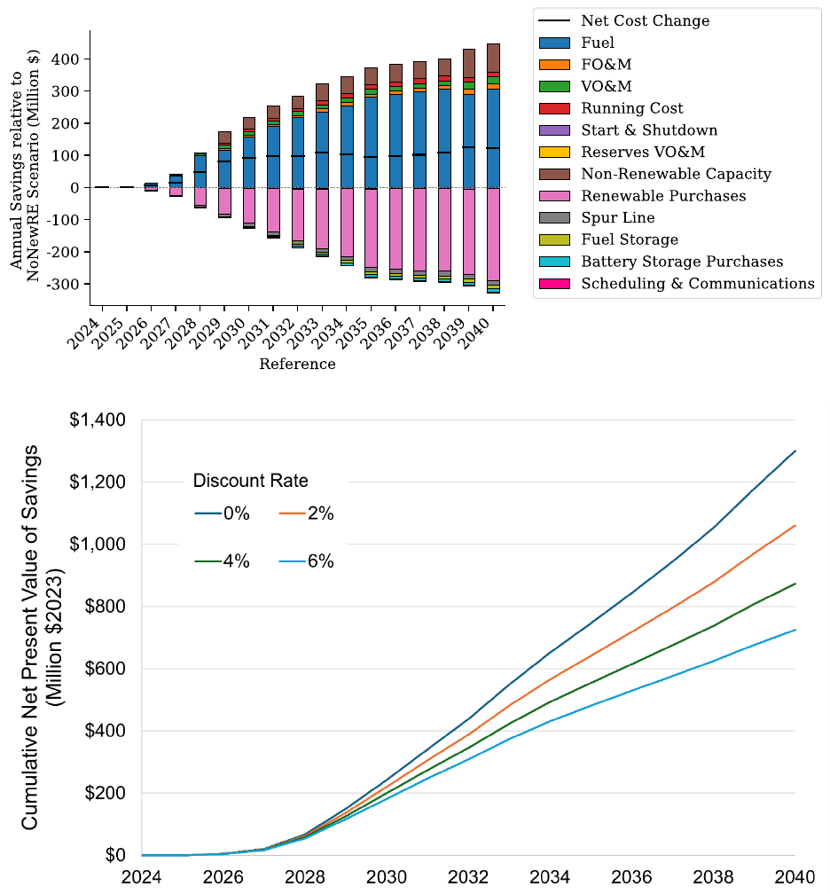
ix
This report is available at no cost from the National Renewable Energy Laboratory (NREL) at www.nrel.gov/publications.
billion. Figure ES-3 (bottom) summarizes the difference in cumulative net present value (NPV)
of evaluated costs over the evaluation period (2024–2040), across a range of discount rates.
Figure ES-3. Total annual savings ($2023) associated with the Reference scenario compared to the
No New RE scenario (top) shows annual savings of about $100 million per year in the early 2030s.
The cumulative (non-discounted) savings from 2024 to 2040 (bottom) reaches $1.3 billion. The net
present value of those cumulative savings is less, depending on discount rate used.

x
This report is available at no cost from the National Renewable Energy Laboratory (NREL) at www.nrel.gov/publications.
Finding #2: The Least-Cost (Reference) Scenario Relies on a Mix of Renewable Energy
Resources and Locations
The Reference scenario deploys a mix of wind and solar resources, with wind providing most of
the new capacity, growing to about 51% of annual generation in 2040. Figure ES-4 shows the
capacity mix (top) and generation mix (bottom) between 2024 and 2040 for the No New RE and
Reference scenarios.
a) Capacity by type
b) Generation by type
Figure ES-4. Capacity (top) and generation mix (bottom) over time in the No New RE and
Reference scenarios
Finding #3: The 80% RPS Has Limited Impact on System Costs, With Much Greater
Uncertainty Driven by Future Costs of Renewables and Other Resources
Adding the RPS requirement has a small impact on the overall savings associated with
deployment of renewable energy compared to the Reference scenario. The Reference (least-cost)
scenario achieves a 76% contribution from renewable resources in 2040. Above this level of
renewable generation, additional renewables have a slightly higher cost than operating existing
gas plants based on the increasing curtailment (unusable generation) of wind and solar during
periods when the supply of renewables exceeds electricity demand. We assume that all
renewable energy must be paid for regardless of whether it is used.

xi
This report is available at no cost from the National Renewable Energy Laboratory (NREL) at www.nrel.gov/publications.
Figure ES-5 shows the annual savings associated with the Reference and RPS scenarios
compared to the No New RE scenario. The Reference (blue) line is the annual savings shown
previously in ES-3 (top). The RPS line shows the reduction in savings associated with the RPS
scenario resulting in about a $19 million cost (or $19 million reduction in benefits compared to
the Reference scenario) in 2040. This is less than a 2% decrease in cumulative savings. Because
the additional cost occurs almost entirely in 2040 and given the significant uncertainty in future
costs of renewables, fossil fuels, load growth, and other factors, there is essentially no
meaningful difference between the Reference scenario and the 80% RPS scenario. For
comparison, Figure ES-5 also shows how changes in the cost of renewables would have a greater
impact on the overall benefits of deploying renewable resources. A 10% reduction in the cost of
renewables (blue line) would increase the cumulative (non-discounted) savings by about $220M
from 2024 to 2040 (to nearly $1.6 billion). Increasing the cost of renewables by 20% (purple
line) reduces the cumulative benefits by about $470 M (to about $900 million).
Figure ES-5. Requiring an 80% RPS reduces net savings associated by deploying renewable
energy by about $19 million in 2040, which is less than a 2% change in cumulative savings.
Overall, these differences are very small given the large uncertainty in future costs of fuels and
renewable generation demonstrated by the much larger impact of a change in the assumed cost
of renewable energy shown in the high- and low-cost renewable energy sensitivities.
These results suggest that any increase in system costs associated with an 80% RPS (compared
to the Reference scenario) are likely to occur well past 2030, when there will be greater
technological certainty and adjustments to RPS targets could be made to ensure least-cost
deployments.
xii
This report is available at no cost from the National Renewable Energy Laboratory (NREL) at www.nrel.gov/publications.
Finding #4: Demand Is Met in All Scenarios, Relying Heavily on Use of Existing Hydro and
Fossil-Fueled Generators During Periods of Low Renewable Output
Wind and solar resources provide significant cost savings by avoiding fuel use in existing
generators, but maintaining reliable operation in these scenarios depends significantly on
continued use of existing hydropower and fossil generators. There are many periods of low wind
and solar output, and these periods can last for many hours. This demonstrates a fundamental
change in how electricity generation is planned, where renewables may provide the majority of
the energy requirements on an annual basis, but with fossil resources providing a larger fraction
of the capacity requirements.
Finding #5: High-RE Systems Will Require Substantial Changes to How the System Is
Operated
The use of highly variable resources will require changes to how the system will maintain
supply-and-demand balance. These changes include increased variation in output from existing
fossil and hydropower plants and variation in transmission flows along the interties. We assume
that planning and operating are performed in a coordinated manner to minimize cost and ensure
resource adequacy and operational reliability across the entire Railbelt system, but that each
utility can operate independently. This kind of operation, including Railbelt-wide joint dispatch,
may require changes to contractual agreements or other practices to minimize the costs of
operating the system.
The system will need to rely increasingly on dispatching wind and solar generators by curtailing
their output (but still paying for the lost energy production at full price). The output from wind
power plants can be controlled over the available output range in less than 1 minute, while the
output from solar can be controlled over its output range in a few seconds. This will be needed to
maintain supply/demand balance but also for the provision of operating reserves from renewable
resources. Although the majority of operating reserves are derived from storage and existing
fossil and hydropower plants, wind and solar may play an increasing role in providing operating
reserves.
Finding #6: Cost Impacts of Addressing Variability and Uncertainty Are Modest Relative
to Savings but With Remaining Uncertainties
All results presented in this analysis include the impact of several factors associated with
integrating renewables and addressing variability and uncertainty, which increases the cost or
reduces the net value of renewable energy. To clarify these changes in costs, Figure ES-6
illustrates how addressing renewable variability and uncertainty impacts the net overall value of
renewable energy seen in the Reference scenario.
The left set of bars shows the total costs of renewable energy purchases and integration. The
bottom (pink) bar is the cost of renewable purchases, which captures all the annual fixed and
variable costs from the wind and solar power plants. By 2040, these direct project costs are about
$285M/year. Additional direct costs assumed for both wind and solar include spur line cost and
substation upgrades, natural gas storage and scheduling, communication, and forecasting, adding
about $27M/year by 2040. Additional factors include the costs associated with additional starts
and stops of power plants, the reduction in avoided natural gas associated with responding to

xiii
This report is available at no cost from the National Renewable Energy Laboratory (NREL) at www.nrel.gov/publications.
variability and uncertainty, and additional operating reserves. These are “embedded” in the
results seen previously, but additional analysis was performed to isolate these costs—which are
estimated at about $18M/year by 2040. Combined, integration-related factors add about
$45M/year in 2040 to the cost of purchasing solar and wind energy.
The right set of bars shows the value of the fuel and variable costs avoided by this generation.
The difference in the total renewables cost (left bars) and avoided costs (right) produce the net
value, which averages about $105 million per year beginning in 2030 as shown in Finding #1.
Figure ES-6. Annual costs of renewable energy, including integrating and addressing resource
variability, are shown in the left set of bars. These costs are included in all scenarios but are
broken out here for clarity. These increase renewable costs by about 16% compared to only the
cost of the renewable generator and interconnection. The right bars show the value of avoided
variable costs, with the difference being the net savings associated with renewable deployment.
These impacts are important not only to accurately assess the value of variable and uncertain
resources but also to consider when allocating system costs across multiple utilities. There is still
considerable uncertainty about some of these factors, particularly natural gas fuel storage.
Additional issues related to maintaining system stability with high levels of inverter-based
resources must also be addressed and may incur additional costs, which can be compared to the
annual savings.
Conclusions and Caveats
The high projected prices for natural gas in the Railbelt region make the addition of renewable
resources potentially cost-competitive despite challenges including development costs, moderate
resource quality, and the small system size, which increase the relative impact of variability and
uncertainty. Based on the assumptions used in this analysis, achieving more than a 75%
contribution of renewables toward Railbelt electricity by 2040 appears to be the least-cost option.
Moving to an 80% RPS slightly decreases the cumulative cost savings that result from
0
50
100
150
200
250
300
350
400
450
500
2024 2025 2026 2027 2028 2029 2030 2031 2032 2033 2034 2035 2036 2037 2038 2039 2040
Annual Costs (Million $2023)
Renewable Purchases Start & Shutdown
Spur Line Scheduling & Communications
NG Fuel Storage
Part-Load Heat Rate
Op. Reserves
Avoided Costs
xiv
This report is available at no cost from the National Renewable Energy Laboratory (NREL) at www.nrel.gov/publications.
renewables deployment (by about 1%) because the mismatch of renewable supply and electricity
demand limits the ability of renewables to displace the remaining fossil generation without
further cost reductions or use of new technologies such as seasonal storage.
There are several significant uncertainties around the scenarios evaluated in this work. Among
them are the potential load growth driven by EVs and the future price of natural gas.
This analysis was conducted based on the information available within timing constraints. It is a
starting point for additional research and consideration of investment or policy options. Other
factors that can inform decision making are not considered here. The analysis results are not
intended to be the sole basis of investment, policy, or regulatory decisions but are rather intended
to improve the understanding of the cost impacts of an 80% RPS. Only direct costs are
measured; other potential benefits of renewable energy such as energy security and reduced
exposure to fuel price volatility are not considered. We also do not consider potential benefits
associated with improved local air quality, which is a concern in several areas of Alaska’s
Railbelt that are at, or nearing, nonattainment status for fine particulate matter (PM
2.5
).
Additional modeling will be required to further validate the findings of this work, including
changes and associated additional costs that are likely needed to ensure stable operation when
nearly all the grid’s electricity is being derived from inverter-based wind, solar, and storage.
xv
This report is available at no cost from the National Renewable Energy Laboratory (NREL) at www.nrel.gov/publications.
Table of Contents
Acknowledgments ..................................................................................................................................... iv
List of Acronyms ......................................................................................................................................... v
Executive Summary ................................................................................................................................... vi
Table of Contents ...................................................................................................................................... xv
List of Figures ......................................................................................................................................... xvii
List of Tables ............................................................................................................................................ xix
1 Introduction ........................................................................................................................................... 1
1.1 Study Goals ................................................................................................................................... 1
1.2 General Approach ......................................................................................................................... 3
1.3 Caveats 3
2 Overview of the Alaska Railbelt System ............................................................................................ 4
3 Modeling Methods and Assumptions ................................................................................................. 7
3.1 Modeling Approach ....................................................................................................................... 7
3.1.1 Capacity Expansion Modeling ......................................................................................... 7
3.1.2 Production Cost Modeling ............................................................................................... 8
3.2 Reliability- and Resource-Adequacy-Related Assumptions ......................................................... 8
3.2.1 Planning and Operation .................................................................................................... 8
3.2.2 Resource Adequacy (Planning Reserve Margin) Assumptions ........................................ 9
3.2.3 Operational Reliability Assumptions ............................................................................... 9
3.3 Addressing Wind and Solar Variability and Uncertainty .............................................................. 9
3.3.1 Increased Cycling and Part-Load Operation of Thermal Plants ..................................... 10
3.3.2 Increased Operating Reserves ........................................................................................ 10
3.3.3 Natural Gas Fuel Storage ............................................................................................... 12
3.3.4 Renewable Curtailment .................................................................................................. 13
3.3.5 Renewable Scheduling and Forecasting ......................................................................... 13
3.3.6 Accommodating Inverter-Based Resources ................................................................... 13
4 Scenarios Evaluated .......................................................................................................................... 13
4.1 Scenario Overview ...................................................................................................................... 13
4.2 RPS Target .................................................................................................................................. 14
4.3 Eligible Technologies .................................................................................................................. 14
4.4 Other Policies .............................................................................................................................. 15
5 Reference Assumptions .................................................................................................................... 16
5.1 Load 16
5.1.1 Load Shape ..................................................................................................................... 16
5.1.2 Prescribed Load Growth, Including Electric Vehicles ................................................... 18
5.2 Generation Resources .................................................................................................................. 19
5.2.1 Existing Generation Resources ...................................................................................... 19
5.2.2 Assumed Base Scenario Retirements and Additions ..................................................... 20
5.3 Transmission ............................................................................................................................... 20
5.4 Fuel Prices ................................................................................................................................... 21
6 New Generator Availability, Cost, and Performance Assumptions .............................................. 24
6.1 Technologies Evaluated .............................................................................................................. 24
6.1.1 Completion Dates ........................................................................................................... 25
6.1.2 Treatment of Customer-Sited Resources ........................................................................ 26
6.2 Cost Assumptions ........................................................................................................................ 26
6.3 Resource Availability and Performance ...................................................................................... 29
6.4 Financing Assumptions ............................................................................................................... 29
6.4.1 Treatment of Tax Credits in the Inflation Reduction Act............................................... 29
6.5 Levelized Cost/PPA Price Summary ........................................................................................... 30
7 Key Findings ....................................................................................................................................... 33
xvi
This report is available at no cost from the National Renewable Energy Laboratory (NREL) at www.nrel.gov/publications.
7.1 Finding #1: The Least-Cost (Reference) Scenario Results in Substantial Deployment of
Renewable Energy and Cost Savings .......................................................................................... 33
7.2 Finding #2: The Least-Cost (Reference) Scenario Relies on a Mix of Renewable Energy
Resources and Locations ............................................................................................................. 36
7.3 Finding #3: The 80% RPS Has Limited Impact on Costs Compared to the Reference (Least-
Cost) Scenario ............................................................................................................................. 40
7.4 Finding #4: Demand Is Met in All Scenarios, Relying Heavily on Existing Hydro and Fossil-
Fueled Generators During Periods of Low Renewable Output ................................................... 41
7.5 Finding #5: Large Contributions of Renewable Generation Will Require Substantial Changes to
How the System Is Operated ....................................................................................................... 43
7.5.1 Increased Ramping and Part-Load Operation of Thermal Plants ................................... 44
7.5.2 Changes in Hydropower Plant Operation ....................................................................... 47
7.5.3 Changes to Intertie Flow ................................................................................................ 48
7.5.4 Renewables Dispatch for Balancing Load and for Reserve Provision ........................... 51
7.6 Finding #6: Cost Impacts of Addressing Variability and Uncertainty Are Modest Relative to
Savings but With Remaining Uncertainties ................................................................................ 53
7.7 Additional Findings ..................................................................................................................... 56
7.7.1 Potential Distributed PV Adoption Must Be Evaluated in the Context of Incentives and
Rate Structure Changes .................................................................................................. 56
7.7.2 The Small Increase in Costs Associated With an 80% RPS Are Largely Because of
Renewable Curtailment .................................................................................................. 59
7.7.3 There May Be Additional Costs or Operational Requirements To Address the Reduced
Role of Synchronous Generation and Increased Contribution of Inverter-Based
Resources ....................................................................................................................... 62
7.7.4 Replacing Retiring Renewables Beyond 2040 Should Be Less Expensive Than
Additional Natural Gas Generation ................................................................................ 63
8 Conclusions ........................................................................................................................................ 64
Appendix A. Capacity- and Energy-Related Terms ........................................................................ 65
Appendix B. Base Modeling Assumptions ...................................................................................... 66
B.1 Utility-Owned Fossil Generators ................................................................................................. 66
B.2 Heat Rate and Start Cost Modeling ............................................................................................. 67
B.3 Treatment of CHP Plants and Other Nonutility-Owned Generators ........................................... 68
B.4 Hydropower ................................................................................................................................. 68
B.5 Other Existing Resources ............................................................................................................ 69
B.6 Electric Vehicle Adoption ........................................................................................................... 70
B.7 Operating Reserves ..................................................................................................................... 71
Appendix C. Generator Cost and Performance Assumptions for New Resources ..................... 73
C.1 Land-Based Wind ........................................................................................................................ 73
C.2 Offshore Wind ............................................................................................................................. 78
C.3 Solar (PV) .................................................................................................................................... 79
C.4 Rooftop and Distributed Solar ..................................................................................................... 79
C.5 Geothermal .................................................................................................................................. 80
C.6 Hydropower ................................................................................................................................. 83
C.7 Biomass and Landfill Gas ........................................................................................................... 85
C.8 Energy Storage ............................................................................................................................ 85
C.9 Summary Cost and Financial Parameters for Renewable Generators and Storage ..................... 87
C.10 New Fossil ................................................................................................................................... 90
xvii
This report is available at no cost from the National Renewable Energy Laboratory (NREL) at www.nrel.gov/publications.
List of Figures
Figure ES-1. Types of energy system costs considered in the analysis, depicted for two of the three
scenarios assessed (Reference and RPS). Because the overall study objective is to estimate
the difference in costs among the three scenarios, common costs are not considered in the
analysis. .................................................................................................................................. vii
Figure ES-2. Contribution of renewable energy to the Alaska Railbelt grid in the Reference and No New
RE scenarios .......................................................................................................................... viii
Figure ES-3. Total annual savings ($2023) associated with the Reference scenario compared to the No
New RE scenario (top) shows annual savings of about $100 million per year in the early
2030s. The cumulative (non-discounted) savings from 2024 to 2040 (bottom) reaches $1.3
billion. The net present value of those cumulative savings is less, depending on discount rate
used. ........................................................................................................................................ ix
Figure ES-4. Capacity (top) and generation mix (bottom) over time in the No New RE and Reference
scenarios ................................................................................................................................... x
Figure ES-5. Requiring an 80% RPS reduces net savings associated by deploying renewable energy by
about $19 million in 2040, which is less than a 2% change in cumulative savings. Overall,
these differences are very small given the large uncertainty in future costs of fuels and
renewable generation demonstrated by the much larger impact of a change in the assumed
cost of renewable energy shown in the high- and low-cost renewable energy sensitivities. .. xi
Figure ES-6. Annual costs of renewable energy, including integrating and addressing resource variability,
are shown in the left set of bars. These costs are included in all scenarios but are broken out
here for clarity. These increase renewable costs by about 16% compared to only the cost of
the renewable generator and interconnection. The right bars show the value of avoided
variable costs, with the difference being the net savings associated with renewable
deployment. ........................................................................................................................... xiii
Figure 1. Types of energy system costs considered in the analysis, depicted for two of the three scenarios
assessed (Reference and RPS). Because the overall study objective is to estimate the
difference in costs among the three scenarios, common costs are not considered in the
analysis. .................................................................................................................................... 2
Figure 2. Map of Alaska’s Railbelt power system ........................................................................................ 6
Figure 3. Summary of study modeling flow ................................................................................................. 7
Figure 4. Daily and seasonal generation profiles for 2018 ......................................................................... 17
Figure 5. Assumed fuel price projection ..................................................................................................... 22
Figure 6. Fuel cost projection for existing fossil-fueled plants using 2022 reported heat rate values ........ 23
Figure 7. Assumed Alaska cost multipliers added to all capital costs and O&M costs for renewable
generators and batteries .......................................................................................................... 27
Figure 8. Assumed overnight capital cost for utility-scale PV and land-based wind. Costs do not include
fuel storage or spur line costs, which are calculated separately. ............................................ 28
Figure 9. Example of assumed cost trajectories for wind and solar assuming a 37% capacity factor for
wind and a 17% capacity factor for solar. Costs (in $2023) are fixed for a 25-year period
from the date of completion and include the 40% ITC. This example represents a small
subset of the complete set of resources and locations available and does not include
additional costs associated with interconnection and addressing resource variability. .......... 30
Figure 10. The assumed PPA price trajectory for wind for a location with a 37% capacity factor. The
black line is the initial cost in constant $2023. The solid lines are the contract costs for
projects constructed in 2026 and 2030 in $2023. The dotted lines are the cost in actual
(nominal) dollars assuming a 2.5% escalator. ........................................................................ 31
Figure 11. Wind LCOE supply curve for 2026 and 2030, including spur line cost and variation in capacity
factor. Costs (in $2023) are fixed for a 25-year period from the date of completion and
include a 40% ITC for both the wind plant and spur line. ..................................................... 32
xviii
This report is available at no cost from the National Renewable Energy Laboratory (NREL) at www.nrel.gov/publications.
Figure 12. Contribution of renewable energy increases to about 76% in the Reference scenario .............. 33
Figure 13. Total annual costs ($2023) in the No New RE and Reference scenarios (top) and the net
savings (bottom) resulting from deployment of renewable energy. This includes only
evaluated costs and not costs common to all scenarios. Color key applies to both figures. Net
savings average about $105 million/year from 2030 to 2040. ............................................... 35
Figure 14. The cumulative (non-discounted) savings from 2024 to 2040 reach $1.3 billion. The net
present value of those cumulative savings is less, depending on discount rate used. NPV of
net savings does not include costs and savings that occur past 2040. .................................... 36
Figure 15. Capacity (top) and generation mix (bottom) over time in the No New RE and Reference
scenarios ................................................................................................................................. 37
Figure 16. Location of wind and solar power plants deployed in the Reference scenario. Wind plants
indicated by location and size. Solar is indicated by the amount deployed in each zone but
not located in any specific location. ....................................................................................... 39
Figure 17. Requiring an 80% RPS reduces the net savings from deploying renewable energy by about $19
million in 2040, which is less than a 2% change in cumulative savings. Overall, these
differences are very small given the large uncertainty in future costs of fuels and renewable
generation demonstrated by the much larger impact of a change in the assumed cost of
renewable energy shown in the high- and low-cost RE sensitivities. .................................... 41
Figure 18. System dispatch during the period of peak demand (a), a period of peak fossil plant output (b),
and a period of minimum wind renewable output (c) demonstrating the reliance on existing
hydropower and fossil generators to provide resource adequacy........................................... 42
Figure 19. Fraction of load met by wind and solar shows dramatic variability on an hourly and daily basis
................................................................................................................................................ 43
Figure 20. An example period in the 2040 Reference scenario with a rapid change in renewable output
and response from hydropower and fossil generators ............................................................ 44
Figure 21. Response of Railbelt fossil fuel generators (orange) to a large reduction in wind and solar
output (gray) on November 4, 2040, in the Reference scenario ............................................. 45
Figure 22. Transition of the Southcentral combined-cycle plant from base load to load-following and
peaking operation ................................................................................................................... 46
Figure 23. Declining capacity factor of Central region combined-cycle plants .......................................... 47
Figure 24. Operation of the Bradley Lake hydropower plant during periods of highly variable renewable
output ..................................................................................................................................... 48
Figure 25. Flow on the Alaska Intertie (black) in 2040 in the Reference scenario depends largely on the
supply of wind (orange) in the GVEA region. Positive numbers represent a flow from GVEA
to the Central region. .............................................................................................................. 49
Figure 26. Regional transmission flows, where positive values represent flows from north to Central (AK
Intertie) and south to Central (Kenai Intertie) ........................................................................ 50
Figure 27. Total annual operating (upward) reserves provision by generator type (top) in the No New RE
and Reference scenarios. Total requirement is the black bar. Reserves requirement by type
for the Reference scenario is shown in the bottom. The same legend applies to all plots. .... 52
Figure 28. Annual fossil plant start costs are about $3 million greater per year by the early 2030s in the
Reference scenario compared to the No New RE scenario .................................................... 53
Figure 29. Annual costs ($2023) of renewable energy, including integration and addressing resource
variability, are shown in the left set of bars. These costs are included in all scenarios but are
broken out here for clarity. These increase renewable costs by about 16% compared to the
cost of only the renewable generator and interconnection. The right (blue) bars show the
value of avoided variable costs, with the difference being the net savings associated with
renewable deployment. .......................................................................................................... 55
Figure 30. Daily natural gas fuel consumption in 2040 .............................................................................. 56
Figure 31. Changes in generation mix between the Reference scenario and DPV sensitivity .................... 57
xix
This report is available at no cost from the National Renewable Energy Laboratory (NREL) at www.nrel.gov/publications.
Figure 32. Changes in annual costs, with the DPV sensitivity (top) showing reduction in required utility
expenditures. The avoided cost associated with the DPV sensitivity (bottom) shows the costs
utilities would have to pay for electricity to replace the DPV. .............................................. 58
Figure 33. Curtailment occurring on a 5-day period in 2030 with annual renewable contribution of 54%
(top) and 2032 (bottom) when the annual contribution of renewables has increased to 64% 60
Figure 34. Annual wind and solar curtailment rate shows a dramatic increase when renewable
contribution exceeds 50%-60% .............................................................................................. 61
Figure 35. Example simplified heat rate curve for the Southcentral combined-cycle generator ................ 68
Figure 36. EV adoptions (top) and Reference scenario charging profiles in 2040 (bottom) ...................... 71
Figure 37. Railbelt wind resource and location of wind site evaluated ...................................................... 74
Figure 38. Assumed LCOE/PPA price projections for utility-scale wind operating with an average) (not
including transmission). The PPA price is fixed (in real $2023) for 25 years from the year of
installation, which corresponds to an escalation at the rate of inflation in nominal dollars. .. 77
Figure 39. CapEx projections for offshore wind (top) and LCOE/PPA price projections assuming a 51%
capacity factor (bottom). Cost assumes underwater transmission line connecting to the HEA
system near Homer. The PPA price is fixed for 25 years from the year of installation. ........ 78
Figure 40. Assumed distributed/rooftop PV adoption in the DPV sensitivity ............................................ 80
Figure 41. Assumed geothermal capital cost (top) and LCOE (bottom) .................................................... 81
Figure 42. Potential locations for geothermal resources in Alaska ............................................................. 82
Figure 43. Location of existing and potential new hydropower resources ................................................. 84
Figure 44. Assumed output profile (fraction of installed capacity) for new run-of-river hydropower ....... 85
Figure 45. Assumed battery cost trajectory ($2023 with a 15 year life) ..................................................... 86
List of Tables
Table 1. Characteristics of Alaska’s Railbelt Utilities .................................................................................. 4
Table 2. 2022 Railbelt Utility Generation Mix ............................................................................................. 4
Table 3. Assumed Railbelt RPS Requirement Based on Proposed Senate Bill 101 ................................... 14
Table 4. Assumed Load Growth Based on Population (before addition of electric vehicles) .................... 18
Table 5. Initial (2024) Generation Resource Mix for the Utilities in Alaska’s Railbelt ............................. 19
Table 6. Supply-Side Technologies Considered ......................................................................................... 25
Table 7. Capacity and Generation by Type in 2040 .................................................................................... 38
Table B-1. Existing Railbelt Fossil Fuel Generators (data as reported to EIA) .......................................... 66
Table B-2. Average Heat Rate for Major Fossil Fuel Generators (producing at least 70 GWh in 2022) ... 67
Table B-3. Existing Railbelt Hydropower Plants ........................................................................................ 69
Table B-4. Monthly Water Budget for Existing Railbelt Hydropower Plants ............................................ 69
Table B-5. Existing Railbelt Renewable Generators .................................................................................. 70
Table B-6. Summary of Operating Reserve Modeling ............................................................................... 72
Table C-1. Location and Performance of Available Wind Sites Evaluated ................................................ 76
Table C-2. Overnight Capital Costs (2023$/kW) ....................................................................................... 87
Table C-3. Fixed Charge Rates, Including the Impact of the ITC .............................................................. 88
Table C-4. PTC Value (2023$/MWh): Applied If the Model Chooses To Take the PTC With the Higher
Fixed Charge Rate .................................................................................................................. 89
Tab
le C-5. Fixed O&M Value (2023$/kW-year) ........................................................................................ 90
Table C-6. CT and CCGT Power Plant Cost Estimates .............................................................................. 91
Table C-7. Capital Cost and Fixed Charge Rate for CT, CC, and Coal Plants ........................................... 92

1
This report is available at no cost from the National Renewable Energy Laboratory (NREL) at www.nrel.gov/publications.
1 Introduction
The Alaska Railbelt utilities face growing challenges associated with the declining supply of
natural gas from the Cook Inlet, with substantial price increases projected. Because of this,
renewable energy in the form of wind and solar is a potentially cost-competitive option to reduce
reliance on natural gas, which in 2022 provided nearly two-thirds of the Railbelt electricity
demand.
This study performs an analysis of the system costs and benefits of adding renewable energy to
the Alaska Railbelt grid. The study is motivated in part by a proposed 80% renewable portfolio
standard (RPS).
3
1.1 Study Goals
The primary goal of this current study is to examine differences in total system costs associated
with deploying various amounts of renewable energy. We examine three main scenarios: 1) a
scenario where no additional renewable energy is added, 2) a reference scenario that develops
the least-cost mix of resources, and 3) an 80% RPS scenario.
The cost framework is conceptually illustrated in Figure 1. In all scenarios, there are many
common costs, shown at the bottom of Figure 1. Because the goal of this study is to compare
differences in costs resulting from different generation mixes, we do not estimate these common
costs.
4
This study examines the elements shown at the top of Figure 1, including all factors that
may vary under different portfolios and listed next.
3
Described in proposed Senate Bill No. 101 33-LS0365\R at https://www.akleg.gov/PDF/33/Bills/SB0101A.PDF.
4
Estimating total costs will be required to determine total revenue requirements and establishing rates and rate
structures across various customer classes.

2
This report is available at no cost from the National Renewable Energy Laboratory (NREL) at www.nrel.gov/publications.
Figure 1. Types of energy system costs considered in the analysis, depicted for two of the three
scenarios assessed (Reference and RPS). Because the overall study objective is to estimate the
difference in costs among the three scenarios, common costs are not considered in the analysis.
Cost considered in the study include the following:
• Capital costs and fixed operations and maintenance (O&M) for all new renewable and
fossil generators. For renewables, this could be obtained via a power purchase agreement
(PPA).
• Cost premiums for siting and operating in Alaska.
• Variable costs associated with all existing plants and new plants, including fuel and
O&M. This includes changes to fossil plant operation because of increased variability
from:
o Impacts of part-load heat rate because of increased cycling and load following
o Additional startup costs of fossil plants.
• Costs associated with integrating new renewable resources, including:
o Additional operating reserves
o Grid-forming inverters
o Additional natural gas fuel storage
o Curtailment
o Scheduling, communication, and forecasting costs
o New transmission spur lines and substation upgrades.
Costs not included are those that are not expected to change across the various scenarios:
• Debt on existing assets and existing PPAs
• Fixed O&M on existing assets
Reference Case
RPS Case
Existing Fossil Generator
Fuel and Variable Costs
Costs that do not vary across scenarios
Costs not
considered
in this study
Costs
considered
in this study
$
New Generator and
Storage Costs
Existing Fossil Generator
Fuel and Variable Costs
New Generator and
Storage Costs

3
This report is available at no cost from the National Renewable Energy Laboratory (NREL) at www.nrel.gov/publications.
• Administrative and billing costs
• 86 MW of energy storage currently proposed or under development
• Distribution system costs
• Maintenance and upgrades of the existing transmission network not associated with new
renewable generators
• Upgrades to the Kenai Intertie associated with the Railbelt Innovative Resiliency Project
• Infrastructure associated with electric vehicles (EVs).
1.2 General Approach
The study follows the traditional principles of least-cost resource planning, sometimes referred to
as integrated resource planning. The study uses a standard commercially available model that
simulates the evolution and operation of the power system to identify the mix of resources that
maintains system reliability at the lowest life cycle cost. It begins with the existing generation
mix and adds new resources it identifies as providing electricity with the lowest overall cost,
considering all fixed and variable costs. The model tracks several reliability metrics, including
the ability to serve demand during all hours of the year, and maintains adequate reserves to
address generator failures. Across the various scenarios, we report differences in generation mix
and costs on both an annualized basis and net present value (NPV).
1.3 Caveats
This analysis was conducted based on the information available within timing constraints. It is a
starting point for additional research and consideration of investment or policy options. Other
factors that can inform decision making are not considered here. The analysis results are not
intended to be the sole basis of investment, policy, or regulatory decisions but are rather intended
to understand the cost impacts of increased renewable deployment, including impacts of an 80%
RPS. Only direct system costs are measured—other potential benefits of renewable energy such
as energy security and reduced exposure to fuel price volatility are not considered. We also do
not consider potential benefits associated with improved local air quality, which is a concern in
several areas of Alaska’s Railbelt that are at, or nearing, nonattainment status for fine particulate
matter (PM
2.5
).
5
5
State of Alaska Department of Transportation & Public Facilities, 2020–2023 Statewide Transportation
Improvement Program (STIP). Approved November 23, 2021, Amendment 3 and Incorporated Administrative
Modifications (State of Alaska Department of Transportation and Public Facilities, 2021).
https://dot.alaska.gov/stwdplng/cip/stip/assets/STIP.pdf
.

4
This report is available at no cost from the National Renewable Energy Laboratory (NREL) at www.nrel.gov/publications.
2 Overview of the Alaska Railbelt System
This analysis applies to Alaska’s Railbelt power system, which extends from Fairbanks through
Anchorage to the Kenai Peninsula and consists of four electric cooperatives and one municipally
owned (not-for-profit) utility that serve about 75% of Alaska’s electricity (Table 1).
6
Table 1. Characteristics of Alaska’s Railbelt Utilities
Data are for 2022 and from U.S. Energy Information Administration (EIA) Form 861.
a
Utility
Annual Sales
(GWh)
Customer
Accounts
(thousands)
Fraction of Railbelt
Annual Demand (%)
Chugach Electric Association
1,903 113
43
Golden Valley Electric Association
1,244 48
28
Matanuska Electric Association
766 69
17
Homer Electric Association
453 33
10
City of Seward Electric Department 53 3 1
Total
b
4,404 266 100
a
“Annual Electric Power Industry Report, Form EIA-861 detailed data files.” EIA,
https://www.eia.gov/electricity/data/eia861/.
b
This does not include about 254 GWh of electricity lost in transmission and distribution plus electricity
consumed by the utility. The total net generation requirement in 2022 was about 4,698 GWh.
Overall, the system obtains the majority of its electricity from fossil resources, summarized in
Table 2.
7
Table 2. 2022 Railbelt Utility Generation Mix
8
Technology
Capacity
(MW)
Energy
(GWh)
Generation
Fraction
Natural gas
1,332.6
3,052
64%
Coal
117.5
545
11%
Oil
268.9
444
9%
Hydropower
189.8
578
12%
Wind
44.5
107
2%
Landfill gas
11.5
41
1%
Total
1,965
4,766
100%
6
This table does not include some of the electricity consumed by large users that supply a portion of their own
demand, including the University of Alaska Fairbanks or military bases.
7
Data do not include the contribution from solar or small hydropower.
8
Totals may not add up to 100% because of rounding. Data from EIA Form 860 and Form 923 for the year 2022.
Only large generators are listed, and this does not include distributed resources. List includes Aurora but not CHP

5
This report is available at no cost from the National Renewable Energy Laboratory (NREL) at www.nrel.gov/publications.
Figure 2 illustrates Alaska’s Railbelt region. Fairbanks is served by the Golden Valley Electric
Association (GVEA). For the purposes of modeling, we combined the Chugach Electric
Association (serving Anchorage), the Matanuska Energy Association (MEA), and the City of
Seward Electric Department into a single zone we refer to as “Central” throughout this study.
The Homer Electric Association (HEA) serves the Kenai Peninsula.
plants at UAF, industrial, or military sites. https://www.eia.gov/electricity/data/eia860/;
https://www.eia.gov/electricity/data/eia923/.

6
This report is available at no cost from the National Renewable Energy Laboratory (NREL) at www.nrel.gov/publications.
Figure 2. Map of Alaska’s Railbelt power system
9
9
Data from Alaska Energy Data Gateway, Electric Service Areas. Alaska Energy Authority, 2020.
https://gis.data.alaska.gov/datasets/DCCED::electric-se
rvice-areas/explore?location=61.907409%2C-
147.863943%2C6.00.

7
This report is available at no cost from the National Renewable Energy Laboratory (NREL) at www.nrel.gov/publications.
3 Modeling Methods and Assumptions
This work studies the period from 2024 to 2040 and follows a standard least-cost planning
approach using models and general assumptions described in this section.
3.1 Modeling Approach
The study uses a modeling approach illustrated conceptually in Figure 3 and described in detail
next.
Figure 3. Summary of study modeling flow
10
3.1.1 Capacity Expansion Modeling
Capacity expansion analysis is the central modeling element of the study because it produces the
generation mix and estimates the total system costs associated with each scenario. Within the
capacity expansion modeling step, the study identifies future generation and transmission
portfolios to achieve renewable energy targets at least cost.
Modeling the expansion of the bulk power system, including utility-scale (noncustomer-sited)
generators and transmission, is performed with the PLEXOS Long-Term Model.
11
The capacity
expansion model (CEM) considers capital costs, fixed and variable O&M costs, and fuel costs,
moving forward in time in 1-year increments over the study period (2024–2040). Investment
decisions for the type, amount, and location of new capacity are determined with a least-cost
optimization that ensures the provision of power system resources required to meet load reliably
in all hours and meets all other constraints and policies.
10
Brinkman, Gregory, Dominique Bain, Grant Buster, Caroline Draxl, Paritosh Das, Jonathan Ho, and Eduardo
Ibanez et al. 2021. The North American Renewable Integration Study: A U.S. Perspective—Executive Summary.
Golden, CO: National Renewable Energy Laboratory. NREL/TP-6A20-79224-ES.
https://www.nrel.gov/docs/fy21osti/79224-ES.pdf
.
11
https://www.energyexemplar.com/plexos.

8
This report is available at no cost from the National Renewable Energy Laboratory (NREL) at www.nrel.gov/publications.
3.1.2 Production Cost Modeling
The production cost model (PCM) is used to simulate the hourly operations of the future systems
identified by the CEM and to validate the ability of those systems to balance generation and
load.
12
We use the PLEXOS Medium-Term/Short-Term model, a commercially available PCM
(sometimes referred to as a unit commitment and dispatch model). This is the same model used
in a previous NREL report that analyzed several aspects of how Alaska’s Railbelt grid might be
operated in 2040 when providing 80% of electricity generation from renewable energy
resources.
13
The system details generated by the CEM (types, capacities, and locations of transmission,
renewable generation, and conventional generation), are passed to the PCM, along with hourly
load and variable generation data and hourly operating reserve requirements.
14
The PCM
calculates operational costs and ensures that adequate reserves are maintained under the given set
of weather and load conditions.
15
This type of simulation is an iterative process. The PCM provides necessary feedback to the
CEM to determine more definitively if the built system can operate feasibly. If PLEXOS
identifies unserved energy (i.e., load that the system is unable to serve) or other constraint
violations (e.g., reserves shortages or hydro violations), the CEM can be refined to incorporate
additional constraints or requirements, which directly impacts the resulting build decisions.
3.2 Reliability- and Resource-Adequacy-Related Assumptions
3.2.1 Planning and Operation
We assume that planning is performed in a coordinated manner to minimize cost and ensure
resource adequacy and operational reliability across the entire Railbelt system. Practically
speaking, this does not require a single entity to plan the system but does require coordination
across the utilities—including likely joint planning of assets, particularly those generation assets
that provide energy to multiple utilities. This process could include joint ownership of plants,
shared PPAs, or any other policy mechanism that maximizes planning efficiency.
Likewise, we assume coordinated system operation (joint dispatch), meaning that the generators
and transmission assets are operated in a manner to produce the overall least systemwide cost,
while maintaining independent reliability in each of the utility zones. We do not include the costs
associated with full system coordination but do include an additional cost in the Reference and
RPS scenarios associated with scheduling and forecasting additional renewable resources (see
12
This model was used in the previous Railbelt study.
13
Denholm, P.; M. Schwarz, E. DeGeorge, S. Stout, and N. Wiltse. 2022. Renewable Portfolio Standard Assessment
for Alaska’s Railbelt. Golden, CO: National Renewable Energy Laboratory. NREL/TP-5700-81698.
14
Operating reserves represent generator capacity available to address variability and uncertainty in generation
supply and demand and include contingency, flexibility, and regulating reserves. Reserves can be held by partially
loaded generators (or offline generators, depending on the type of reserve) with sufficient ramp to respond in a given
time frame.
15
NREL often evaluates subhourly variability, but insufficient data were available to consider the impact of
increased subhourly variability in this study; instead, we used estimates for operating reserve requirements needed to
address ramp rate requirements within the hour.

9
This report is available at no cost from the National Renewable Energy Laboratory (NREL) at www.nrel.gov/publications.
Section 3.3.5). This study did not assume any specific regulatory approach that might achieve
this type of operation, and this does not require utilities to merge or otherwise lose independence
to ensure local reliability and rate setting.
We assume that each utility zone can be islanded and operated in isolation and maintain
resource adequacy. During islanded operation, the 80% RPS requirement is not enforced.
3.2.2 Resource Adequacy (Planning Reserve Margin) Assumptions
We require sufficient capacity to reliably serve load during all hours of the year, including times
of system stress, which are often peak-load or peak-net-load
16
conditions—of which the
magnitude and timing are uncertain. The total firm capacity requirement is typically defined as
expected peak load in each year plus a predetermined generation capacity margin (the planning
reserve margin) for reliability. Based on previous Railbelt utility studies, we maintain a 30%
planning reserve margin in each zone, meaning that installed dependable capacity must be at
least 30% higher than the expected peak demand in each year.
17
The capacity must be located
within the zone, so imports on the interties do not count toward the planning reserve margin.
Firm capacity differs from total nominal or nameplate capacity—it is the portion of nominal
capacity that is reliably available during times of system stress. We assume that all existing
thermal and hydropower plants are eligible to contribute to the planning reserve margin. The
ability of wind and solar resources to serve peak demand (capacity credit; see Appendix A) is
substantially lower than those of hydropower and thermal assets and described in the technology
discussions in Appendix C.
3.2.3 Operational Reliability Assumptions
We require operating reserve to ensure that there is sufficient capacity that can quickly vary
output to 1) address unexpected generator or transmission line outages; 2) respond to short-term
random variation in load, wind, and solar output; and 3) balance out longer-term (up to 1 hour)
uncertainty and forecast errors in net load, including ramping.
18
We require contingency
spinning reserves to address rapid failures of large plants or transmission lines (80 MW) and
regulating reserves (2% of load in Central and HEA and 5% in GVEA) to address rapid and
unpredictable variations in load. We also include additional operating reserves to address the
variability of wind and solar (see Section 3.3.2). Further description is provided in Appendix
B.7.
3.3 Addressing Wind and Solar Variability and Uncertainty
The variability and uncertainty of wind and solar can create changes in how the system is
planned and operated. These changes are sometimes considered in terms of an “integration cost,”
16
The concept of “net load” is commonly used in systems with large amounts of renewable resources and refers to
the normal load minus the contribution of wind and solar. This is important because it determines the amount of
hydropower, fossil, or other resources needed to ensure reliability.
17
See section 8.1 in the 2010 Alaska Railbelt Regional Integrated Resource Plan (RIRP) 2010.
https://www.akenergyauthority.org/Portals/0/Publications%20and%20Resources/2010.02.01%20Alaska%20Railbelt
%20Integrated%20Resource%20Plan%20(RIRP)%20Study.pdf?ver=2022-03-22-115635-150.
18
See Table B-6 for further discussion of treatment of operating reserves.

10
This report is available at no cost from the National Renewable Energy Laboratory (NREL) at www.nrel.gov/publications.
although there is no clear definition of what these costs are or how to quantify them.
19
In some
scenarios, they may be direct hardware costs associated with the installation of individual
renewable energy projects. These costs are captured in the project costs as modeled, and for
wind, include the costs of transmission interconnections. Many historical integration costs
studies focused on the change in value of renewable energy as it is deployed compared to more
traditional generation sources.
20
Overall, we capture the impact of wind and solar on the overall system cost via the simulation of
systems with and without the addition of renewable energy. The following subsections discuss
how we consider six general categories of impact, including the potential changes to system
costs.
3.3.1 Increased Cycling and Part-Load Operation of Thermal Plants
Renewable energy resources can reduce the amount of variable costs associated with operation
of fossil-fueled power plants, including fuel, O&M, and starts. As an example, a 2013 National
Renewable Energy Laboratory (NREL) study of wind and solar providing 33% of the electricity
in the western United States found that inclusion of thermal plant cycling reduces the value of
renewable resources by $0.1–$0.7/MWh (in $2011).
21
As the net load variability increases, thermal plants will spend a greater fraction of time
operating at part load and with an increased number of generator starts. Power plants operating at
part load are less efficient than at full load, meaning that their average heat rate under scenarios
with more wind and solar may increase. This tends to somewhat reduce the overall benefits of
wind and solar. This impact is captured using heat rate curves, which measure how the
performance of the plants changes as a function of generation.
The net benefits of wind and solar may also be reduced from the increased number of thermal
plant starts. During startup, power plants require additional fuel to spin up the turbine and
synchronize it to the grid and incur costs associated with wear and tear, increased maintenance,
and other direct costs. Values for start fuel requirements and other costs were obtained from the
Railbelt utilities and other sources described in Appendix B.2.
3.3.2 Increased Operating Reserves
Wind and solar add variability to net load across multiple time scales and with various degrees of
uncertainty. To address variability and uncertainty of wind and solar, we add operating reserves.
Operating reserves causes three changes to system planning and operation that increase the costs
(or decrease the value) of wind and solar. The first is if new capacity resources are required
specifically to address the operating reserve requirements. The second change is less-efficient
19
Michael Milligan, Erik Ela, Bri-Mathias Hodge, Brendan Kirby, Debra Lew, Charlton Clark, Jennifer DeCesaro,
and Kevin Lynn. 2011. “Integration of Variable Generation, Cost-Causation, and Integration Costs.” The Electricity
Journal 24(9): 51–63. ISSN 1040-6190. https://doi.org/10.1016/j.tej.2011.10.011
.
20
A. D. Mills, R. H. Wiser, “Changes in the economic value of photovoltaic generation at high penetration levels: A
pilot case study of California” in 2012 IEEE 38th Photovoltaic Specialists Conference (PVSC) (2012), pp. 1–9.).
21
Lew, D., Brinkman, G., Ibanez, E., Florita, A., Heaney, M., Hodge, B. M., Hummon, M., Stark, G., King, J.,
Lefton, S. A., Kumar, N., Agan, D., Jordan, G., and Venkataraman, S. Western Wind and Solar Integration Study
Phase 2. United States: 2013. Web. doi:10.2172/1095399. https://www.nrel.gov/docs/fy13osti/55588.pdf.

11
This report is available at no cost from the National Renewable Energy Laboratory (NREL) at www.nrel.gov/publications.
dispatch.
22
Because more “headroom” is needed to increase output, thermal plants will spend
more time operating at partial load, and there will be greater use of batteries to provide reserves
(meaning that they cannot be used to provide other services), or the system may require more
curtailed wind and solar (decreasing their ability to offset fossil generators).
23
The third change
is additional cycling of power plants responding to subhourly variability. In combination, these
impacts result in a reduction in avoided costs compared to a scenario where an increase in
operating reserves is not required.
The amount of reserves needed as a function of wind and solar deployment varies significantly
based on the size of the system.
24
In large systems, a relatively small increase is required—often
just a small percentage of the combined output of wind and solar. This is because of the impact
of spatial variability, which smooths the combined output of a diverse supply of resources. As
the system decreases in size, there is less diversity, and the net ramp rates increase. There are
limited studies of reserve requirements for a system the size of Alaska.
25
Based on the relatively
small size of the Alaska system and limited data available, we assume a much higher level of
reserves compared to Lower 48 utility systems.
26
Operating reserves are required primarily to
address the unpredictable portion of the wind and solar variability or to address variability that
occurs faster than normal system scheduling and dispatch. We make the conservative assumption
that wind ramp events are essentially unforecastable in the subhourly time frame.
Based on this assumption, the available wind and solar data sets require maintaining sufficient
operating reserves to accommodate a 60% change in output from the aggregated wind resources
in each zone in less than 30 minutes. We meet this requirement in the form of two operating
reserve products. The first is a traditional rapid-response regulating reserve product from a
synchronized generator or energy storage equal to at least 20% of wind output that addresses the
short-term (<10-minute) variability. The second reserve product (supporting 40% of wind
output) is a slower (<30-minute) flexible ramping product used to address the longer-term
variability. This product has been used in a variety of locations in the Lower 48 as a lower-cost
alternative to addressing solar and wind variability only with fast-responding units. With a
combination of reserve products, initial response to an unforecasted ramping event is from the
22
Hummon, M., P. Denholm, J. Jorgenson, D. Palchak, B. Kirby, and O. Ma. 2013. Fundamental Drivers of the
Cost and Price of Operating Reserves. Golden, CO: National Renewable Energy Laboratory. NREL/TP-6A20-
58465.
23
This is sometimes referred to as the “opportunity cost” of providing reserves particularly in regions with
wholesale markets because a unit providing reserves cannot sell energy losing the opportunity to increase revenue.
24
P. L. Denholm, Y. Sun, and T. T. Mai. 2019. An Introduction to Grid Services: Concepts, Technical
Requirements, and Provision from Wind. Golden, CO: National Renewable Energy Laboratory. NREL/PR-6A20-
73590. https:/doi.org/10.2172/1505934.
25
The Hawaii Electric system is somewhat close in size and physically small, which reduces opportunities for
spatial diversity. However, this system has very different load patterns, and most renewable capacity is in the form
of solar—so likely of limited value. An example study of this system is
https://www.ferc.gov/sites/default/files/2020-08/W3B-3_Ela.pdf
.
26
NREL typically calculates reserve requirements by examining the size of unforecastable ramp events from
potential combinations of new wind and solar generators. This requires detailed subhourly data sets, which were not
available for this study. For additional discussion, see https://www.nrel.gov/docs/fy14osti/61016.pdf
.

12
This report is available at no cost from the National Renewable Energy Laboratory (NREL) at www.nrel.gov/publications.
faster regulating reserves (which begin responding in a few seconds or less), and sustained
longer ramps are then addressed by flexibility reserves.
27
We also require 30% of online solar to be supported by operating reserves (20% from fast-
responding regulating reserves and 10% by a flexible ramping reserve).
28
In addition to these
requirements, we maintain the 80 MW of fast contingency reserve response, even when the
largest thermal generator online is less than this amount. This means that during periods of the
highest level of wind and solar contribution, we exceed the 60% requirement.
Note that operating reserves are not intended to balance supply and demand over longer (multi-
hour) time periods or provide energy during periods of low wind and solar output. Maintaining
service during periods of low wind and solar output is accomplished via the planning reserve
margin, which establishes resource adequacy.
3.3.3 Natural Gas Fuel Storage
The Alaska Railbelt system depends on a limited natural gas pipeline supply network and has
limited storage capability. This may increase the challenge of responding to net load variability
using the existing natural gas power plant fleet. Deploying renewable energy will decrease the
average natural gas consumption rate. However, it can increase the changes in consumption rate
(flow rate in the natural gas supply system), and the actual supply needed is less predictable. This
presents challenges to how the system is scheduled as well as the technical capacity of the
system to vary the supply of natural gas. To address this challenge, Railbelt utilities are
considering the addition of natural gas fuel storage, acting as a buffer to address the increased
variability and uncertainty of natural gas demand. To capture this, we included the cost of fuel
storage required to supply natural gas fuel for thermal generation entirely from storage for 99%
of all 24-hour periods, assuming a 40% forecast error in renewable resources. We note that this
quantity of storage does not ensure deliverability and further analysis is required to ensure the
variability in demand can be met. The capital cost of new aboveground fuel storage is assumed
to be $2.5/cubic foot, which we assume is not eligible for the investment tax credit (ITC) and
financed at the same rate as a new gas plant.
29
This cost is applied proportionally to all additional
renewable capacity based on the average contribution of all renewables to the increased
variability of natural gas demand.
30
27
P. L. Denholm, Y. Sun, and T. T. Mai. 2019. An Introduction to Grid Services: Concepts, Technical
Requirements, and Provision from Wind. Golden, CO: National Renewable Energy Laboratory. NREL/PR-6A20-
73590. https:/doi.org/10.2172/1505934.
28
We do not require operating reserves to address longer-term solar ramps driven by sunrise and sunset because
these are predictable and addressed via ramp constraints in the system dispatch. The model ensures that the available
generation capacity can ramp to meet predictable hourly ramps in the same manner as predictable changes in load.
29
Note that this is the capital cost, not the variable cost of fuel storage. The costs are based on correspondence with
Chugach, reporting a value of $30 million for 12 million cubic feet of storage. Note that because we apply these
costs as a proportion of renewable capacity, this implies a continuous deployment of incremental amounts of gas
storage, while actual deployment would likely occur in larger discrete projects to take advantage of economy of
scale.
30
This cost can potentially be compared to the cost of existing underground storage provided by Cook Inlet Natural
Gas Storage Alaska. For example, see 2023 Expansion Inception Rates at
https://aws.state.ak.us/OnlinePublicNotices/Notices/View.aspx?id=213184
. These costs are quoted on a per unit

13
This report is available at no cost from the National Renewable Energy Laboratory (NREL) at www.nrel.gov/publications.
3.3.4 Renewable Curtailment
The impact of renewable curtailment on overall value is included in the analysis. All potential
renewable energy production must be paid for at full price regardless of whether it is used.
Although curtailment of wind generation would produce a small reduction in O&M costs, this
value is not included.
3.3.5 Renewable Scheduling and Forecasting
We add a system scheduling, communications, and forecasting cost of renewables once wind and
solar provide more than 20% of annual generation. The assumed cost is $1.5 million/year based
on scheduling tariffs from ISO-NE.
31
Note that this does not include all the costs associated with
establishing joint dispatch including investments in software, communication systems, and
training. Joint dispatch would provide benefits even without the additional renewables and is
assumed in all scenarios—including the No New RE scenario—and the benefits of joint dispatch
are not isolated to compare to potential additional costs.
3.3.6 Accommodating Inverter-Based Resources
Large deployment of inverter-based resources including solar, wind, and battery plants can result
in decommitting (turning off) thermal and hydropower resources that use synchronous
generators. This can reduce the inherent inertial response and provision of fault current available
in the grid in addition to other services that stabilize the system. To replace these services,
several options are possible, including the use of grid-forming inverters, other power-electronics-
based options, increased transmission capacity, or use of synchronous machines, including
synchronous condensers, which includes modifying existing generators to act as synchronous
condensers. A combination of approaches is likely; note that the cost-optimal mix of these
resources has not been identified. For the purposes of the analysis, we assume that grid-forming
inverters will be deployed as part of the solution to maintain stability. We therefore require all
new wind solar, wind, and battery plants to have grid-forming inverter capabilities in the year at
which instantaneous contribution of inverter-based resources in any region during any point in
the year hits 50%. We assume a 20% cost premium over grid-following inverters. We also
compare potential overall savings to additional measures that may be necessary, including the
use of dedicated new synchronous condensers.
4 Scenarios Evaluated
4.1 Scenario Overview
We evaluated three scenarios for comparison. The first scenario (referred to as No New RE) does
not allow for any new renewable construction. The second (Reference) is a reference scenario
actually stored as opposed to the cost of physical capacity. To make this comparison, we would need to understand
the actual utilization of energy storage in the future, which would require a greater understanding of the forecast
error in wind and solar power production and the actual storage withdrawals, and we do not have good estimates.
However, assuming a range of utilization between 10% and 20% per day, the assumed cost of $2.5/cubic foot capital
cost would correspond to a variable cost of about $3–$6/MCF.
31
https://www.iso-ne.com/static-assets/documents/regulatory/tariff/sect_4/section_iva.pdf.

14
This report is available at no cost from the National Renewable Energy Laboratory (NREL) at www.nrel.gov/publications.
without an RPS requirement and represents the overall least-cost mix of resources. The third
(RPS) enforces the RPS trajectory. Two sensitivities are also performed for the Reference and
RPS scenarios, which examine the impact of higher and lower renewable resource costs. Each
scenario maintains the same minimum planning reserve margin requirement.
4.2 RPS Target
The RPS in this study approximates the proposed policy in Senate Bill 101.
32
Table 3
summarizes the RPS targets, defined as fraction of annual generation (not sales).
33
The RPS as
modeled in this analysis is defined as a target for the entire Railbelt and is not enforced for
individual utilities. This formulation of the RPS implies frictionless trading of renewable
resources between zones via renewable energy certificates (RECS) or other mechanisms and
would require appropriate allocation of costs associated with integration and balancing among
the participants. We do not extend REC trading beyond the Railbelt, and we assume full
compliance with the RPS.
34
We also did not consider other possible policy options such as credit
banking.
35
We do not consider requirements that may occur after 2040 but discuss potential cost
trends that may occur after 2040 in Section 7.7.4. The RPS scenario we evaluate requires
sufficient generation capacity to meet 80% of annual generation after considering the
deliverability of each renewable resource because of transmission congestion, losses in storage,
and curtailment resulting from oversupply during periods of high renewable energy output or
low electricity demand.
Table 3. Assumed Railbelt RPS Requirement Based on Proposed Senate Bill 101
Year Value
2027 25%
2035 55%
2040 80%
The RPS target is enforced in the planning process and not during system operation, including
periods of extended outage condition.
36
There is no preference for dispatch of RE resources
during operation on any basis other than variable cost.
4.3 Eligible Technologies
We assume that RPS-eligible technologies include wind, solar, geothermal, tidal, hydropower,
biomass, and landfill gas and include both existing and new deployments. The SB101 language
32
https://www.akleg.gov/PDF/33/Bills/SB0101A.PDF.
33
Our study assumes that the RPS requirement must be met for the year listed and so is more aggressive than the
SB101 requirement, which sets the target the last day of each year.
34
The current bill includes a $20/MWh compliance penalty, but we assume full compliance to determine the actual
cost associated with additional renewables.
35
For additional discussion of RPS design and features, see Renewable Portfolio Standards, NREL,
https://www.nrel.gov/state-local-tribal/basics-portfolio-standards.html.
36
We assume that achieving the RPS is contingent on normal operation of the interties but that maintaining
reliability is not. Average outage rate on the intertie from 2012 to 2021 was about 1.3%.
https://www.akenergyauthority.org/Portals/0/RailBeltEnergy/IMC/2022/2022.05.20/8A.%20%20AlaskaIntertieStrat
egicPlanningUpdate%202022-05-20%20rev0.pdf?ver=2022-05-19-133503-887.
15
This report is available at no cost from the National Renewable Energy Laboratory (NREL) at www.nrel.gov/publications.
includes energy efficiency; however, this was not included in the analysis because of lack of data
(amount and cost of savings and impact on load shape).
4.4 Other Policies
We include all federal policies, including the investment and production tax credits as currently
modeled in the NREL 2023 Annual Technology Baseline (ATB) (discussed in detail in Section
6.4.1). We assume no other changes to state policies, meaning:
• No state carbon pricing or other policies
• No changes to state air quality standards or emission control requirements/emissions fees.

16
This report is available at no cost from the National Renewable Energy Laboratory (NREL) at www.nrel.gov/publications.
5 Reference Assumptions
The study began with the development of a power system model of the existing Alaska Railbelt
system that could be used as an initial starting point for the 2024 simulation year. After
establishing a base system, we developed a set of assumed changes that are common across
scenarios, including load growth and certain resource additions and retirements between 2024
and 2040. Note that throughout this report, all data we share is from publicly available data
sources.
5.1 Load
5.1.1 Load Shape
For each of the three zones (GVEA, Central, and HEA, shown in Figure 2), we first established
an initial load shape.
37
Hourly load shapes are based on 2018 because it corresponds to the
availability of simulated wind resource data. These hourly load profiles form the basis for the
total generation requirement in each region (considering transmission and distribution losses).
Figure 4 provides examples of the hourly load profiles in each of these regions, which varies as a
function of time of day and season. Figure 4(a) shows daily load profiles in 2018 for the Central
region (combining Chugach Electric Association, MEA, and Seward), GVEA, and HEA in the 4-
day period with highest (systemwide) annual demand, which occurred during the hour ending at
7 p.m. on January 25. Figure 4(b) shows the total systemwide demand for this period as well
as for the periods with the lowest systemwide demand in October and the highest systemwide
summer demand in July.
38
The Railbelt system is strongly winter-peaking.
39
37
Data provided by AEA.
38
Maximum and minimum demand periods for individual utilities may be different from those for the overall
system. Note that the terms generation, load, and demand throughout this report refer to the generation required to
serve the end-use demand plus transmission losses. Therefore, numbers will generally be about 6% higher on
average compared to actual sales to end customers. This reflects transmission and distribution losses.
39
The strong winter peak makes it easier to analyze the potential contribution from solar toward resource adequacy
and operational reliability. For this study, we assume it is zero, unlike in summer-peaking systems where
photovoltaics (PV) contribution can be significant but requires detailed analysis of time-coincident output of solar
energy and demand peaks.

17
This report is available at no cost from the National Renewable Energy Laboratory (NREL) at www.nrel.gov/publications.
(a) Winter peak generation for three modeled utility regions: Central, GVEA, and HEA
(b) Total generation in three periods in Alaska’s Railbelt
Figure 4. Daily and seasonal generation profiles for 2018
0
50
100
150
200
250
300
350
400
450
500
1/24/18 12:00 AM 1/25/18 12:00 AM 1/26/18 12:00 AM 1/27/18 12:00 AM 1/28/18 12:00 AM
Railbelt Generation (MW)
Central
HEA GVEA
0
100
200
300
400
500
600
700
800
12:00 AM 12:00 PM 12:00 AM 12:00 PM 12:00 AM 12:00 PM 12:00 AM 12:00 PM 12:00 AM
Railbelt Generation (MW)
Winter Peak (Jan 24-28) Fall Minimum (October 12-14) Summer Peak (July 31-Aug 3)

18
This report is available at no cost from the National Renewable Energy Laboratory (NREL) at www.nrel.gov/publications.
5.1.2 Prescribed Load Growth, Including Electric Vehicles
To account for load growth, demand profiles were scaled based on regional population growth
estimates from the Alaska Department of Labor and Workforce Development.
40
Estimated
population growth is about 4.5% across the entire Railbelt from 2021 to 2040 but with significant
variation regionally. This scaling resulted in an annual generation requirement of about 4.76
TWh in 2024 (the initial study year) and 4.86 TWh in 2040 (Table 4).
41
Peak generation grows
from 735 MW in 2024 to 763 MW in 2040. No change in load shape from different electricity
use patterns or weather is assumed, and we do not assume changes to load shape because of
addition or retirement of large industrial loads. We also do not assume any additional energy
efficiency, demand response, or load flexibility measures.
Table 4. Assumed Load Growth Based on Population (before addition of electric vehicles)
Region
Generation Requirement
Total Increase
(%)
2024 2040
Central 2,972 3,132 5.4%
Golden Valley Electric Association 1,242 1,264 1.8%
Homer Electric Association 473 464 -1.8%
Total
a
4,686 4,860 3.7%
a
Totals may not add up to 100% because of rounding.
In addition to load growth based on population, we added a base level of EV adoption using data
gathered by the Alaska Center for Energy and Power.
42
For the Reference scenario, we used the
most conservative (lowest) growth level, from the “AEA continued” forecast, which results in
about 110,000 vehicles (about 20% of all vehicles in the Railbelt) in 2040 (additional details
provided in Appendix B.6).
43
The total increase in generation requirements by 2040 is about
16% (782 GWh, including a transmission and distribution [T&D] loss multiplier of 1.057).
44
EV
charging is assumed to be unmanaged, so potentially significant benefits of controlled charging
are not included.
40
https://live.laborstats.alaska.gov/pop/projections/pub/popproj.pdf.
41
Actual generation requirement in 2022 was about 4.7 TWh (see Table 1), so this results in a 10% increase from
2022 to 2040.
42
Cicilio, P.; Francisco, A.; Morelli, C.; Wilber, M.; Pike, C.; VanderMeer, J.; Colt, S.; Pride, D.; Helder, N.K.
Load, Electrification Adoption, and Behind-the-Meter Solar Forecasts for Alaska’s Railbelt Transmission System.
Energies 2023, 16, 6117. https://doi.org/10.3390/en16176117 https://www.mdpi.com/1996-1073/16/17/6117
.
43
ACEP provides two other adoption scenarios that were not used in this report, including a “moderate” forecast,
which assumes 150,000 EVs in 2040 (30% of all vehicles) and adds another 367 GWh of load, or an “aggressive”
forecast, which roughly doubles EV adoption by 2040.
44
This is based on an average 5.4% T&D loss factor based on a 2022 Railbelt average from EIA form 860.

19
This report is available at no cost from the National Renewable Energy Laboratory (NREL) at www.nrel.gov/publications.
5.2 Generation Resources
5.2.1 Existing Generation Resources
A database of existing plants was derived from Railbelt utilities and publicly available data
sources.
45
There are some small differences between the data shared in this document related to
existing power plant performance and the data we use in the model databases (where we defer to
utility-provided data sets). We also assume a total of 16.9 MW of distributed solar installed by
the end of 2023 based on Alaska Center for Energy and Power (ACEP) estimates.
46
Table 5
summarizes the systemwide capacity and mix for the initial 2024 conditions.
Table 5. Initial (2024) Generation Resource Mix for the Utilities in Alaska’s Railbelt
47
Key parameters required for modeling the operation of these existing plants include capacity (see
Appendix A), operating costs (fuel, variable O&M, and startup costs). Fuel costs are the product
45
“Form EIA-860 Detailed Data with Previous Form Data (EIA-860A/860B),” EIA,
https://www.eia.gov/electricity/data/eia860/.
“Form EIA-923 Detailed Data with Previous Form Data (EIA-906/920),” EIA,
https://www.eia.gov/electricity/data/eia923/.
46
Generation of DPV would be typically captured in load profiles. Because we are using 2018 data with limited PV
adoption, we add DPV profiles separately. In 2022, utilities had about 2,200 customers, with 13.2 MW of PV under
“net metering,” of which 11 MW was residential (EIA 860). Projections for the end of 2023 (adding about 3.7 MW
of distributed PV) are from ACEP Cicilio, P.; Francisco, A.; Morelli, C.; Wilber, M.; Pike, C.; VanderMeer, J.; Colt,
S.; Pride, D.; Helder, N.K. Load, Electrification Adoption, and Behind-the-Meter Solar Forecasts for Alaska’s
Railbelt Transmission System. Energies 2023, 16, 6117. https://doi.org/10.3390/en16176117
https://www.mdpi.com/1996-1073/16/17/6117
.
47
Location represents the physical location and does not consider the regional allocation of energy from various
resources, such as the share of Bradley Lake allocated to utilities outside of the HEA region.
Generator Type
Capacity (MW)
HEA Central GVEA Total
Combustion turbine (CT) 124 424 0 548
Internal combustion (IC) 0 165 0 165
Combined cycle (CC) 80 366 60 506
Oil steam 18 0 185 203
Coal steam 0 0 93 93
Hydropower 120 59 0 179
Wind 0 18 25 43
Landfill gas 0 7 0 7
Solar (utility-scale plus distributed) 3 12 19 34
Energy storage 46 0 40 86
Total 391 1,143 535 2,069

20
This report is available at no cost from the National Renewable Energy Laboratory (NREL) at www.nrel.gov/publications.
of the price of fuel and the heat rate (fuel consumed per unit of generation). Fuel prices are
discussed in Section 5.4. Other data are from plant-level data provided by the utilities or from a
similar plant when not provided. Heat rate data include impact of part-load operation.
We also consider operating constraints for all plants, including operating range (minimum
output), minimum on/off time (hours the plant must stay on once turned on, or hours the plant
must stay off once turned off), and ramp rate (how quickly the plant can change output).
48
Fixed costs of existing assets, including fixed O&M and outstanding debt payments, are not
considered because these are the same in all scenarios. Changes in O&M associated with
increased cycling in response to renewable deployment is captured by the variable costs,
particularly the increased annual number of starts and associated costs. Appendix B provides a of
every generation resource assumed in the initial 2024 system, including treatment of power plant
efficiency and hydropower operation.
5.2.2 Assumed Base Scenario Retirements and Additions
In addition to capacity that existed on January 1, 2024, we assume near-term additions of two
battery plants currently planned for completion in the near future. We assume a 40-MW/2-hr
system in the Central region completed at the beginning of 2025 and a 46-MW/2-hr system in
GVEA completed at the beginning of 2026 (which replaces the existing 15-minute system).
Costs of these new facilities are not considered because they are included in all scenarios. There
are several proposed wind and solar plants;
49
these were not included so we could fully account
for the costs of new renewable capacity, including balancing and integration.
Most of the existing capacity is retained through the 2040 study period. Based on feedback from
Railbelt utilities, we assume retirement only of Healy Unit 2 in 2025.
5.3 Transmission
Our model aggregated Alaska’s Railbelt power system into three transmission zones, illustrated
in Figure 2. Transmission is not modeled within each of the three zones. All five utilities are
electrically interconnected, which allows the utilities to exchange resources and thus improve the
economic operation of the grid. However, the connection between GVEA and the utilities to the
south via the Alaska Intertie is limited; also limited are the connections to HEA through the
Kenai Intertie (see Figure 2 for the location of these interties). Because transmission outages can
occur, these regions must be able to operate independently.
48
Although we allow combined-cycle plants to operate over their full range (with a simplified heat rate curve that
captures operation over multiple modes), we require all starts to assume the mode of operation with the longest start
time and with the highest start costs. Our assumption substantially reduces the operational flexibility of the plants
and their ability to quickly start individual gas turbines when responding to unforecasted changes in wind and solar.
This conservative assumption is intended to offset some of the limitations created by the lack of forecast error in the
wind, solar, and load data sets.
49
For example: https://aws.state.ak.us/OnlinePublicNotices/Notices/View.aspx?id=206903.

21
This report is available at no cost from the National Renewable Energy Laboratory (NREL) at www.nrel.gov/publications.
Between each zone, we represent the interties using the following assumptions in all scenarios:
• Alaska Intertie: Runs from Healy to Willow. We assume 78 MW of available transfer
capacity
50
and a 6% loss rate on transfers on the existing AK Intertie.
51
We do not consider
any potential upgrades to the Alaska Intertie, so the maximum transfer limit stays at 78 MW
over the time frame of the study.
• Kenai Intertie: Runs from Soldotna to Quartz Creek and is currently rated at about 75 MW
of capacity, and we assume an 8% loss rate.
52
We assume that it is upgraded to 185 MW of
capacity in 2033 as part of the Railbelt Innovative Resiliency Project.
53
The cost of intertie
upgrade is not considered because it applies to all scenarios.
54
The only other changes to the transmission network are interconnections for new wind where
costs vary with distance and size, as discussed in Appendix C.1. For the rest of the T&D system,
we assume that average historical loss rates do not change (these losses are embedded in the total
generation profiles).
5.4 Fuel Prices
Figure 5 shows assumed fuel price projection in $2023.
55
Prices for natural gas in the near term
are from the AEA and assume a transition to liquified natural gas (LNG) imports.
56
We assume
that LNG becomes available in 2028 and establishes the avoided cost of all natural gas purchases
starting in that year. The initial cost assumed of gas (delivered to the point of use) is
$12.1/MMBtu in $2023,
57
and we also assume a 0.5%/year real price increase and that fuel
prices are constant throughout each year. We do not consider the potential impacts of fuel price
volatility and the potential benefits of renewable energy to provide bill stability via long-term
fixed cost contracts. We also note that there is considerable uncertainty about the various options
available for future natural gas supplies and cost.
50
Ongoing studies by AEA and others have considered an upgrade to the Alaska Intertie; however, this has not been
considered in this study. For example, a possible increase to 195 MW of capacity and reduction of losses to about
3%. From: Alaska Intertie Strategic Planning Update, May 20, 2022.
https://www.akenergyauthority.org/Portals/0/RailBeltEnergy/IMC/2022/2022.05.20/8A.%20%20AlaskaIntertieStrat
egicPlanningUpdate%202022-05-20%20rev0.pdf?ver=2022-05-19-133503-887.
51
The loss rate will actually vary as a function of flow on the line; however, we use a simplified average loss rate
based on Figure 4.1 in the 2010 RIRP.
52
Also a simplified average loss rate based on Figure 4.1 in the 2010 RIRP.
53
This upgraded capacity value is based on the Railbelt Innovative Resiliency Project application “Battery Energy
Storage/HVDC Coordinated Control,” which states, “studies indicate the southern transfer limit could likely be
increased by over 150%,” which results in a capacity of at least 185 MW.
54
The project received $413M in funding.
55
Prices for fuel oil and initial price of natural gas from AEA “Alaska Energy Authority Renewable Energy Fund
Program Round 14 November 16, 2021.” Prices for coal from GVEA filings - Compilation of GVEA Usibelli Coal
Invoices and assumes a small real (above inflation) increase based on AEA projections.
56
Discussion of declining natural gas production from Cook Inlet is provided by
https://dog.dnr.alaska.gov/Documents/ResourceEvaluation/Cook_Inlet_Gas_Forecast_Report_2022.pdf.
57
https://www.enstarnaturalgas.com/wp-content/uploads/2023/06/CIGSP-Phase-I-Report-BRG-28June2023.pdf.

22
This report is available at no cost from the National Renewable Energy Laboratory (NREL) at www.nrel.gov/publications.
Figure 5. Assumed fuel price projection
Figure 6 shows the fuel costs translated into generation cost ($/MWh) for the six fossil fuel
plants that provided more than 90% of all fossil generation on the Railbelt in 2022 (and more
than 75% of all generation).
58
Figure 6a shows costs for the four natural-gas-fueled plants in the
Central region that provided the most significant generation in 2022. Figure 6b shows a coal and
an oil-fired combined-cycle (CC) plant in the GVEA region. These curves do not show the costs
of running peaking and backup plants that can have significantly higher fuel costs but rarely run.
58
See Appendix B for 2022 generation and heat rate data.
$0
$2
$4
$6
$8
$10
$12
$14
$16
$18
$20
$22
$24
2024 2026 2028 2030 2032 2034 2036 2038 2040
Fuel Price (2023$/MMBTU)
Fuel Oil Coal Natural Gas

23
This report is available at no cost from the National Renewable Energy Laboratory (NREL) at www.nrel.gov/publications.
a) Natural gas (Central and HEA regions)
b) Coal and fuel oil (GVEA region)
Figure 6. Fuel cost projection for existing fossil-fueled plants using 2022 reported heat rate values
$0
$20
$40
$60
$80
$100
$120
2024 2026 2028 2030 2032 2034 2036 2038 2040
Fuel Cost Using Historical Heat Rate
($2023/MWh)
Eklutna Sullivan/Southcentral Nikiski
$0
$20
$40
$60
$80
$100
$120
$140
$160
$180
2024 2026 2028 2030 2032 2034 2036 2038 2040
Projected Fuel Cost using Historical
Average Heat Rate (2023$/MWh)
North Pole CC
Coal (Healy)
24
This report is available at no cost from the National Renewable Energy Laboratory (NREL) at www.nrel.gov/publications.
6 New Generator Availability, Cost, and Performance
Assumptions
This section provides an overview of cost and performance assumptions. Additional details,
including tables of costs and financial parameters, are provided in Appendix C.
6.1 Technologies Evaluated
Table 6 lists generation options considered.

25
This report is available at no cost from the National Renewable Energy Laboratory (NREL) at www.nrel.gov/publications.
Table 6. Supply-Side Technologies Considered
Technology Notes
Fossil
Coal and Gas Cogeneration Not considered with exceptions noted
Conventional Coal Existing and new
Combined Cycle (CCGT) Existing and new
Combustion Turbine Existing and new
Internal Combustion Engine Only existing capacity
59
Oil/Gas Steam Only existing capacity
Renewables
Biomass (solid biomass
combustion)
No (preliminary analysis indicated that this would not
be competitive)
Geothermal New capacity at a single location after 2030
Hydropower Existing plants plus new run-of-river; no new
conventional hydro
Landfill Gas Only existing capacity
Land-Based Wind Existing and new (only utility-scale)
Offshore Wind New capacity after 2030 in the Cook Inlet
Rooftop PV Only existing capacity in base scenario; prescribed
builds as a sensitivity
Tidal No
Utility-Scale PV Existing and new
Storage
Battery Storage Existing and new
Pumped Storage Hydro No
60
Technologies not listed are not considered, including fossil with carbon capture and storage, small modular nuclear,
or hydrogen fuels.
6.1.1 Completion Dates
All new generation capacity is assumed to be completed and available at full capacity at
midnight on January 1 of the year it enters service. This assumption applies to all other changes
59
Internal combustion units may have some advantages over new CT or CCGT capacity not captured in this study,
as discussed in Appendix C.9.
60
We did not have sufficient cost and performance data to evaluate pumped storage hydropower, but previous
analysis indicates that there are several potentially suitable sites for pumped storage. See Koritarov, V., Meadows,
R., Kwon, J., Esterly, S., Balducci, P., Heimiller, D., DeGeorge, E., Stout, S., Clark, C., Ingram, M., Desai, J., and
Rosenlieb, E. The Prospects for Pumped Storage Hydropower in Alaska. United States: N. p., 2023. Web.
doi:10.2172/1987825. https://publications.anl.gov/anlpubs/2023/07/183313.pdf.

26
This report is available at no cost from the National Renewable Energy Laboratory (NREL) at www.nrel.gov/publications.
to the model as well, so all prescribed builds, retirements, and load growth occur at midnight on
January 1.
6.1.2 Treatment of Customer-Sited Resources
Rooftop and distributed solar are eligible to contribute toward the RPS in SB101. Modeling
distributed solar, including costs and benefits, is challenging because of the many assumptions
needed about adoption rates and estimates of possible cross-subsidies from the utility to the
customers, from customers to the utility, or across customer classes. Analysis needs to consider
how rate structures may evolve, and the impact of feed-in tariffs or net metering regulations.
Prior analysis of distributed solar adoption by NREL has been performed using the agent-based
dGen adoption model; however, this model has not been applied to Alaska.
61
To avoid the need to quantify the impact of net metering regulations and associated costs, in the
base scenario we assume that all solar after 2024 is deployed or acquired by the utility at the
costs described in Appendix C.3. We assume a total of 16.9 MW of distributed solar installed by
the end of 2023 (discussed previously), but after this point there is no new distributed solar
deployment by utility customers in the Railbelt. This means that all costs associated with new
solar are borne by the utility and there are no cross-subsidies. Although this allows for an easier
direct comparison across scenarios, a scenario with zero distributed solar adoption is unrealistic.
Therefore, we also developed a distributed solar sensitivity scenario. We use projections from
ACEP using its moderate forecast, which assumes about 210 MW of rooftop solar by 2040, with
trajectory provided in Figure 41 in Appendix C.
We do not consider the impact of customer-sited storage or wind. Distributed wind is common in
Alaska, although more common in remote locations.
62
Future analysis could consider the impact
of these technologies but with the same caveats regarding the need to analyze rate structures,
revenue requirements, and potential cross-subsidies.
6.2 Cost Assumptions
For most renewable technologies and storage, we used projections of the costs and performance
from NREL’s 2023 Annual Technology Baseline.
63
For each technology, the ATB provides
projections of future costs (including capital, financing, grid connection, and fixed and variable
O&M) from present day to 2050 and reflects representative conditions in the Lower 48 states.
Costs include all components needed to install and interconnect the generator to the local grid
but not spur line costs, which must be added separately. Costs in the ATB are reported in $2021,
which is inflated to $2023 for this study using an inflation factor of 1.12.
64
For this study, we
used the mid cost projections from the ATB, and we then applied a technology-specific
multiplier to all fixed and variable cost components. This factor is applied to all regions and
reflects an overall mix of Alaskan conditions, including generally higher costs of transportation
61
https://www.nrel.gov/analysis/dgen/.
62
https://www.energy.gov/sites/default/files/2022-08/distributed_wind_market_report_2022.pdf.
63
https://atb.nrel.gov/.
64
Price escalators from the CPI: https://www.usinflationcalculator.com/inflation/consumer-price-index-and-annual-
percent-changes-from-1913-to-2008/.

27
This report is available at no cost from the National Renewable Energy Laboratory (NREL) at www.nrel.gov/publications.
and construction and relatively immature markets (meaning limited vendors and developers in
Alaska). For less mature technologies (those with limited deployment in Alaska), the multiplier
decreases over time. Figure 7 shows the assumed multipliers applied to ATB capital and O&M
costs. The decline is partially a result in the assumption of a maturing market that would likely
require sustained deployment of these technologies over many years. Note that these values
apply to the initial cost of an individual project and do not decline for that project after it is
installed.
Figure 7. Assumed Alaska cost multipliers added to all capital costs and O&M costs for renewable
generators and batteries
Figure 8 shows capital cost assumptions for wind and solar, reported in 2023$/kW
ac
. Values for
other technologies are provided in Appendix C. The lower (dotted) lines represent projections for
the Lower 48 region from the ATB where a decline in costs is expected based on declining
installed costs and operating costs.
65
The Alaska (solid) lines are the product of the ATB costs
and Alaska multiplier.
66
65
Wiser, Bolinger et al. LBNL, U.S. Department of Energy Office of Energy Efficiency and Renewable Energy.
Land-Based Wind Market Report: 2021 Edition. http://www.osti.gov.
66
The U.S. EIA uses a wind multiplier of 1.3 in Anchorage and 1.56 for wind in the Fairbanks region.
(https://www.eia.gov/analysis/studies/powerplants/capitalcost/pdf/capcost_assumption.pdf). We assume that it will
take 10 years of deployment to achieve a mature market in Alaska.
1
1.1
1.2
1.3
1.4
1.5
1.6
1.7
1.8
1.9
2024 2026 2028 2030 2032 2034 2036 2038 2040
Alaska Capital Cost Multiplier
Year of Installation
Wind Geothermal/Run of River Hydropower PV Batteries
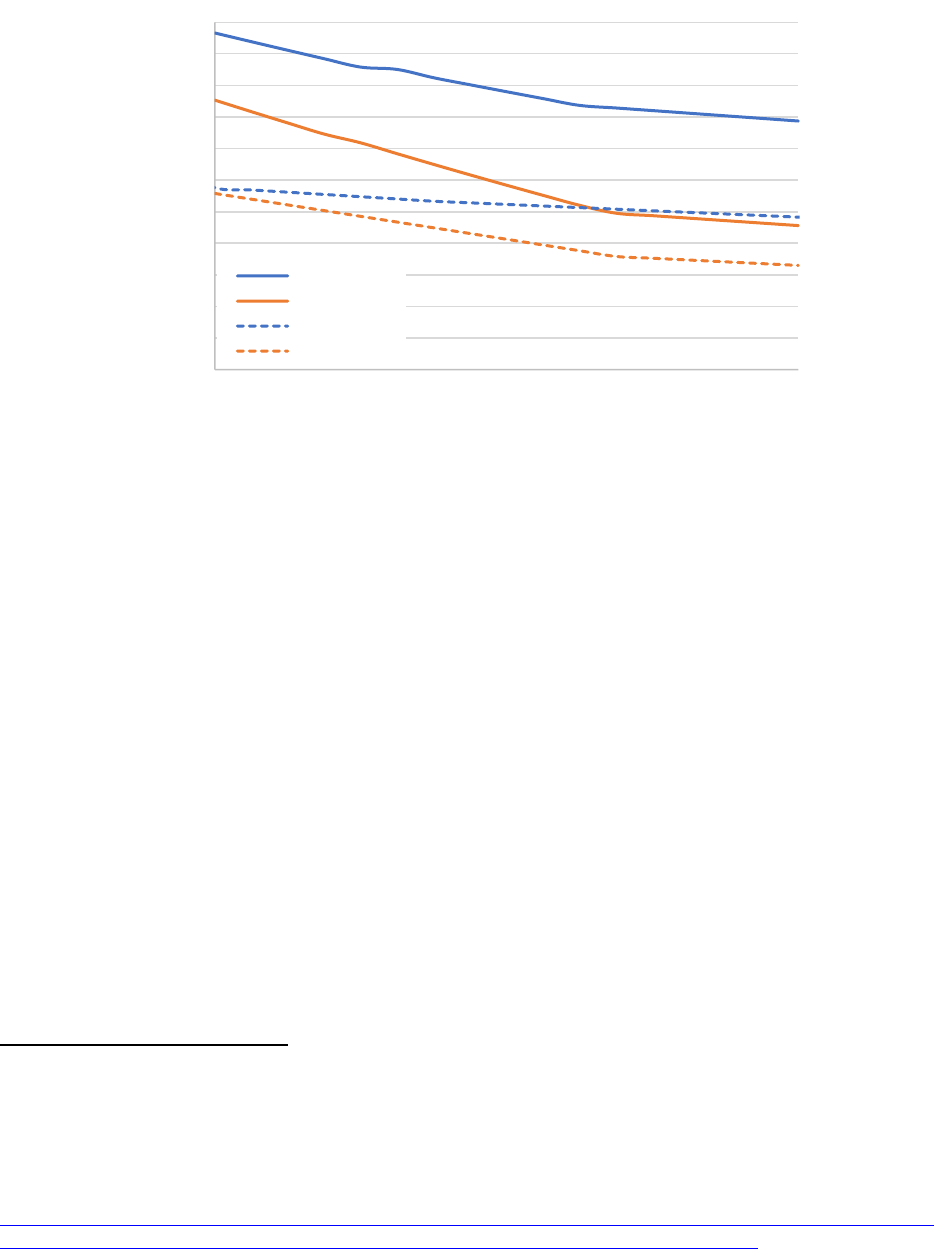
28
This report is available at no cost from the National Renewable Energy Laboratory (NREL) at www.nrel.gov/publications.
Figure 8. Assumed overnight capital cost for utility-scale PV and land-based wind. Costs do not
include fuel storage or spur line costs, which are calculated separately.
Spur line costs are added for wind, geothermal, and PV, assuming a blended average distance-
based spur line cost of $11/kW-km (and assumed to be eligible for the ITC), with distance by
technology discussed in Appendix C. Additional substation upgrades for wind and solar projects
are assumed to add $25/kW and are assumed to not be eligible for the ITC.
67
We also perform two cost sensitivities, where the low-cost sensitivity applies a 10% cost
reduction to all renewable energy technologies and a high-cost sensitivity increases renewable
energy costs by 20%.
For cost of new fossil fuel resources, we relied primarily on the 2010 Regional Integrated
Resource Plant (RIRP) study
68
and adjusted to $2023 to account for inflation and technology
improvements based on trends observed from EIA Annual Energy Outlook (AEO).
69
A further
cost reduction between 2023 and 2040 is based on the ATB 2023 projections, assuming
continued technology improvements. Capital costs tend to be higher than NREL ATB values,
likely reflecting higher Alaska construction costs, but also demonstrating the impact of smaller
unit size, reducing economy-of-scale benefits.
67
Substation costs are derived from Lopez, A. et al. 2024. Solar Photovoltaics and Land-Based Wind Technical
Potential and Supply Curves for the Contiguous United States: 2023 Edition. NREL/TP-6A20-
87843.https://www.nrel.gov/docs/fy24osti/87843.pdf. We applied a 1.5 Alaska multiplier to the highest cost
values in Table 9 and adjusted to $2023.
68
https://www.akenergyauthority.org/Portals/0/Publications%20and%20Resources/2010.02.01%20Alaska%20Railbelt
%20Integrated%20Resource%20Plan%20(RIRP)%20Study.pdf?ver=2022-03-22-115635-150.
69
Although the ATB provides more recent cost estimates for large fossil fuel plants in the Lower 48, the RIRP study
has detailed analysis of the Alaska-specific costs of developing new fossil-fueled plants.
$0
$250
$500
$750
$1,000
$1,250
$1,500
$1,750
$2,000
$2,250
$2,500
$2,750
2024
2026 2028 2030 2032 2034 2036 2038 2040
Overnight Capital Cost ($2023/kW)
Year of Installation
Wind (Alaska)
PV (Alaska)
Wind (lwr 48)
PV (lwr 48)

29
This report is available at no cost from the National Renewable Energy Laboratory (NREL) at www.nrel.gov/publications.
6.3 Resource Availability and Performance
The performance of wind and solar depends highly on geographical region. For wind, we applied
a land suitability screen and identified 37 sites with a total of about 2,900 MW of capacity, with
methods described in detail in Appendix C.1.Hourly performance was simulated at each location,
and the annual average capacity factor was between 31% and 43% with a fleet average of 36%.
For solar, we used solar profiles generated for four locations in Alaska using both tracking and
fixed-tilt systems, assuming a 1.5 DC/AC ratio. The annual capacity factor, based on the
system’s AC rating, is about 15%–17%.
70
6.4 Financing Assumptions
The analysis used a standard project financing approach, as is typical in integrated resource
planning. For each technology, annual fixed and variable cost components are calculated. The
annual fixed component includes the overnight capital cost multiplied by a fixed charge rate. The
fixed charge rate is derived from multiple factors, including the cost of capital, capital recovery
period, construction time, interest rate, and inflation and is described in detail in the 2023 ATB.
A table of fixed charge rates used for each technology is provided in Appendix C.8.
We do not prescribe an ownership or development model. These plants could be developed by
the individual utilities or acquired via a PPA.
71
This implies that the total cost of ownership
(measured by either NPV or levelized cost of energy [LCOE]) would be the same in both
approaches. The fixed charge rate is the same each year, resulting in an annual payment that is
constant in $2023 (real dollars), which means that it increases in actual (nominal) dollars at the
rate of inflation. This is similar to current PPA structures with escalation clauses, but in this case
the escalation clause changes based on inflation rates.
If acquired via a PPA, the off-taker (utility) must take all energy generated for the purposes of
cost recovery. This means that energy may be curtailed during operation to maintain
supply/demand balance, but curtailed energy must still be paid for.
6.4.1 Treatment of Tax Credits in the Inflation Reduction Act
A variety of technologies are eligible for tax credits as part of the Inflation Reduction Act (IRA).
Most eligible technologies installed in 2025 or later have the option of choosing the production
tax credit or the investment tax credit. For the purposes of calculating a constant (levelized) cost
of energy from various resources, the production tax credit value is levelized using financial
parameters described in the ATB; however, the net result is a value of about $21.5/MWh (in
$2023). This is less than the current (non-levelized) value of $27.5/MWh.
72
The base investment
tax credit is 30% and 40% in certain locations defined as “energy communities.”
73
We assume
that the Railbelt is eligible for the 40% ITC. Projects may also be eligible for a higher ITC value
70
The relatively high capacity factor is a result of the high DC/AC ratio of 1.5. The DC capacity factor is about 13%.
71
The cost of the power purchase agreement (in $/MWh) is calculated using a set of equations described in detail in
the tab labeled “Financial Definitions” in the 2023 ATB spreadsheet. The LCOE equation is at the top of the page.
72
https://www.epa.gov/green-power-markets/summary-inflation-reduction-act-provisions-related-renewable-energy.
73
https://arcgis.netl.doe.gov/portal/apps/experiencebuilder/experience/?id=a2ce47d4721a477a8701bd0e08495e1d

30
This report is available at no cost from the National Renewable Energy Laboratory (NREL) at www.nrel.gov/publications.
if using domestically sourced content, but we make the more conservative assumption of the
lower ITC value.
The model is allowed to choose whichever incentive (ITC or PTC) minimized cost as allowed by
current regulations. The tax credits remain available to the end of the 2040 study period.
74
6.5 Levelized Cost/PPA Price Summary
Figure 9 provides an example of the assumed initial PPA price in constant $2023 for a subset of
technologies, where the date represents the year the project enters into service. The costs for
wind and solar decline over time because of technology improvements and market maturity
following the curves shown in Section 6.2. These costs do not include transmission
interconnections for wind—or the requirements to address variability and uncertainty including
fuel storage and operating reserves, which are also calculated separately—with details provided
in Appendix C.
Figure 9. Example of assumed cost trajectories for wind and solar assuming a 37% capacity factor
for wind and a 17% capacity factor for solar. Costs (in $2023) are fixed for a 25-year period from
the date of completion and include the 40% ITC. This example represents a small subset of the
complete set of resources and locations available and does not include additional costs
associated with interconnection and addressing resource variability.
The values in Figure 9 represent the initial cost of energy assuming a 25-year contract, meaning
that the cost of energy stays constant (in $2023). Figure 10 illustrates the translation between
constant (real) dollars and nominal (actual) dollars using the wind price curve from Figure 9 as
an example. The black line is the same initial cost curve in constant $2023. The solid lines are
74
We assume that the tax credits will begin to phase out in 2038, based on when the Mid-case of the National
Renewable Energy Laboratory's 2022 Standard Scenarios reaches the Inflation Reduction Act of 2022's emissions
reduction targets (Gagnon et al. 2022). However, because of “safe harbor” provisions, we assume that they remain
available for projects completed by January 1, 2040 (the last date we assume that new projections are completed in
this analysis).
$0
$10
$20
$30
$40
$50
$60
$70
$80
$90
2024 2026 2028 2030 2032 2034 2036 2038 2040
Renewabl e LCOE/PPA over a 25-yea r
term (2023 $/MWh)
Year of Project Completion
Solar (17% CF)
Win d (37 %C F)

31
This report is available at no cost from the National Renewable Energy Laboratory (NREL) at www.nrel.gov/publications.
the contract costs for projects constructed in 2026 and 2030 in $2023. Therefore, for a project
completed in 2026, the utility would pay about $63/MWh (solid blue line) for all generation
(including curtailed generation) from the project in $2023 for the next 25 years. The dotted lines
are the cost in actual (nominal) dollars assuming a 2.5% escalator. Therefore, the initial contract
price on January 1, 2026, would be at $68/MWh increasing by 2.5% each year after. In 2030, the
cost of wind is assumed to decrease by about 10% in real ($2023) dollars, but this decline is
offset by inflation, so the initial cost in nominal dollars in 2030 is about the same as in 2026.
This same escalation in nominal dollars would apply to other technologies including solar.
75
Figure 10. The assumed PPA price trajectory for wind for a location with a 37% capacity factor.
The black line is the initial cost in constant $2023. The solid lines are the contract costs for
projects constructed in 2026 and 2030 in $2023. The dotted lines are the cost in actual (nominal)
dollars assuming a 2.5% escalator.
The combination of variation in wind resources plus spur line costs means a range of costs,
particularly for wind. Figure 11 shows the amount of wind deployable at various costs for 2026
and 2030 (in $2023), in the form of a supply curve. This curve includes the spur line costs, which
are assumed to be eligible for the 40% ITC, but it does not include natural gas storage and other
integration needs, which are calculated separately and included in the full results shown in the
following sections.
75
For comparison, the PPA price for the Houston (Alaska) solar project is 6.7 cents/kWh with a 1.5%/year escalator
clause, while we assume a 2.5% escalation http://rca.alaska.gov/RCAWeb/ViewFile.aspx?id=5F71A11E-BC9D-
457A-AD43-B6F765243017.
$0
$10
$20
$30
$40
$50
$60
$70
$80
$90
$100
2024 2026 2028
2030 2032 2034 2036
2038
2040
Wind LCOE/PPA Price ($/MWh)
Year
2026 Nominal
2026 Real
2030 Nominal
2030 Real
Initial Cost in Real Dollars ($2023)

32
This report is available at no cost from the National Renewable Energy Laboratory (NREL) at www.nrel.gov/publications.
Figure 11. Wind LCOE supply curve for 2026 and 2030, including spur line cost and variation in
capacity factor. Costs (in $2023) are fixed for a 25-year period from the date of completion and
include a 40% ITC for both the wind plant and spur line.
0
10
20
30
40
50
60
70
80
0 500 1,000 1,500 2,000 2,500 3,000
Wind LCOE/PPA Price (2023$/MWh)
Cumulative Wind Capacity (MW)
2026
2030

33
This report is available at no cost from the National Renewable Energy Laboratory (NREL) at www.nrel.gov/publications.
7 Key Findings
7.1 Finding #1: The Least-Cost (Reference) Scenario Results in
Substantial Deployment of Renewable Energy and Cost Savings
In the future evolution of the Railbelt power system, the primary driver for economic
deployment of new renewables is their ability to reduce the fuel and other costs of operating
existing fossil generators. After adding the costs of transmission interconnection, natural gas fuel
storage, and other measures needed to address variability, the model identifies wind and solar
resources that have lower life cycle costs than running existing natural gas plants as early as
2025, particularly because the model foresees the increase in natural gas costs occurring in 2028.
Additional wind and solar resources achieve breakeven conditions in subsequent years, and by
about 2030, many of the potential wind and solar resources in the Railbelt region have lower
costs than operating any existing gas plant in the system.
As a result, the model chooses to build large amounts of wind and solar to reduce overall costs.
Figure 12 shows the contribution of renewable energy in the No New RE and Reference
scenarios. In the No New RE scenario, the contribution (as a fraction of generation) decreases
slowly as load grows. In the Reference scenario, the contribution of renewables increases greatly
because of their ability to provide electricity at costs that are lower than the cost of running
existing gas plants, even including costs required to address variability and uncertainty (see Key
Finding #6). The growth in renewable deployment slows considerably in the mid-2030s (when
its contribution reaches about 75%) as the ability of renewables to cost-effectively offset
additional natural gas use drops because of integration challenges, discussed in Section 7.7.2.
The Reference scenario reaches a 76% contribution from renewables by 2040.
Figure 12. Contribution of renewable energy increases to about 76% in the Reference scenario
34
This report is available at no cost from the National Renewable Energy Laboratory (NREL) at www.nrel.gov/publications.
Figure 13 compares the evaluated costs in these scenarios, meaning the total of all costs that may
vary across the different scenarios. As discussed previously, these costs do not include common
costs, such as outstanding debt, existing or planned transmission (including the Kenai Intertie
upgrade), and all costs associated with the distribution system. The common costs would be in
addition to these costs. Figure 13 (top) shows the evaluated annual cost components in constant
$2023. The left curve shows the No New RE scenario, with costs increasing steadily because of
both load growth and fuel cost increases, and fuel purchases exceeding $350 million/year by the
late 2020s. The right curve shows the Reference scenario, showing the significant reduction in
fuel costs and increase in renewable purchase costs. The reduction in fuel costs includes the
impacts of addressing variability of the resources, including additional operating reserves and
thermal plant cycling—including startup and shutdown costs, discussed in more detail in Finding
#6.
Figure 13b shows the difference between the two scenarios, with savings shown as a positive
value and costs shown as negative. The increase in renewable energy purchases is more than
offset by the decrease in fuel-related costs, which produces a net savings (black line) of over
$100 million/year by the early 2030s.

35
This report is available at no cost from the National Renewable Energy Laboratory (NREL) at www.nrel.gov/publications.
a) Annual cost (non-discounted)
b) Annual savings (non-discounted)
Figure 13. Total annual costs ($2023) in the No New RE and Reference scenarios (top) and the net
savings (bottom) resulting from deployment of renewable energy. This includes only evaluated
costs and not costs common to all scenarios. Color key applies to both figures. Net savings
average about $105 million/year from 2030 to 2040.

36
This report is available at no cost from the National Renewable Energy Laboratory (NREL) at www.nrel.gov/publications.
The Reference scenario avoids about $4.2 billion in fuel and other expenses from 2024 to 2040.
This avoided cost requires renewable purchases and other costs of about $2.9 billion, resulting in
a cumulative (non-discounted) savings from 2024 to 2040 in the Reference scenario of about
$1.3 billion. Figure 14 summarizes the cumulative NPV of savings over the evaluation period
(2024–2040), using a range of discount rates. Note that this considers only costs and benefits that
occur prior to 2040, and many of these costs and benefits will continue to accrue past 2040.
76
The values in Figure 14 should not be compared to the full life cycle costs of projects with costs
and benefits that continue past 2040.
Figure 14. The cumulative (non-discounted) savings from 2024 to 2040 reach $1.3 billion. The net
present value of those cumulative savings is less, depending on discount rate used. NPV of net
savings does not include costs and savings that occur past 2040.
7.2 Finding #2: The Least-Cost (Reference) Scenario Relies on a Mix
of Renewable Energy Resources and Locations
The Reference scenario deploys a mix of wind and solar resources, with wind providing the
majority of new capacity. Figure 15 shows the capacity mix (top) and generation mix (bottom)
between 2024 and 2040 for the No New RE and Reference scenarios. The generation mix
excludes curtailed wind and solar energy; however, the costs of curtailed energy are included.
76
Any comparison between the full cost of a project and the values in Figure 14 will omit a large fraction of the
costs and benefits. In the most extreme example, the values in Figure 14 capture only a few percent of the costs and
benefits of projects installed in 2040 because it includes only a single year. Any comparison of additional projects
should use annualized values and compare those annualized values to those in Figure 13.

37
This report is available at no cost from the National Renewable Energy Laboratory (NREL) at www.nrel.gov/publications.
a) Capacity by type
b) Generation by type
Figure 15. Capacity (top) and generation mix (bottom) over time in the No New RE and Reference
scenarios
Table 7 shows the mix of capacity and energy contributions in 2040, with wind providing about
59% of Railbelt electricity in 2040. A map showing wind deployments by area is provided in
Figure 16.. Only land-based wind was deployed in the Reference scenario, driven by the higher
cost of offshore wind, combined with the limited transmission capacity needed to deliver this
energy into the Central zone. Offshore wind projects will have to be relatively large to achieve
the assumed costs, and large offshore wind plants will often exceed spare capacity on the Kenai
Intertie—even with upgrades (see Key Finding #6).

38
This report is available at no cost from the National Renewable Energy Laboratory (NREL) at www.nrel.gov/publications.
Table 7. Capacity and Generation by Type in 2040
Technology
Type
No New RE Reference
Capacity
(MW)
Annual
Energy
(GWh)
Annual
Energy
(%)
Capacity
(MW)
Annual
Energy
(GWh)
77
Annual
Energy
(%)
Fossil 1,673 5,100 86% 1,473 1,442
24%
Land-Based
Wind
43 76
1%
1,400 3,058
51%
Solar 34 42 1% 577 776
13%
Hydropower 179 653
11%
179 629
11%
Other
Renewables
7 55 1% 7 36
1%
Storage
(net
generation)
133 20
(-4)
270 102
(-19)
Total 2,068 5,926 100% 3,905 5,941 100%
Figure 16 provides the quantity of deployed wind and solar power plants in each zone. More
wind is deployed in the GVEA and HEA zones, due to higher quality resources. Solar is added
primarily in the central zone. However, we also note that the quality of the solar data available
for Alaska is relatively poor and may not reflect actual regional variability of the resource that
could alter regional siting.
77
Generation values are after removing curtailment (which must still be paid for). Curtailment of generators is based
on marginal cost. For plants with zero generation cost (wind and solar), plants taking the ITC will be curtailed
before those taking the PTC.

39
This report is available at no cost from the National Renewable Energy Laboratory (NREL) at www.nrel.gov/publications.
Figure 16. Capacity of wind and solar power plants deployed in each zone in the Reference
scenario.
40
This report is available at no cost from the National Renewable Energy Laboratory (NREL) at www.nrel.gov/publications.
7.3 Finding #3: The 80% RPS Has Limited Impact on Costs Compared
to the Reference (Least-Cost) Scenario
Adding the RPS requirement has a small impact on the overall results because the Reference
(Least-Cost) scenario achieves a 76% contribution from renewable resources in 2040. The
installed capacity mix in the RPS scenario is nearly identical to the Reference scenario before
2040, and there are then small differences in 2040. The most significant is the additional 50 MW
of geothermal capacity installed in 2040. Geothermal is likely chosen because a greater fraction
of its production occurs when it can be used, compared to wind and solar, which experience high
levels of incremental curtailment and unusable generation at increased levels of deployment—
which is discussed in more detail in Section 7.7.2.
The difference in cumulative savings between the Reference scenario and the RPS scenario is
less than 2%. Based on the assumptions used in this work and given the significant uncertainty in
future costs of renewables, fossil fuels, load growth, and other factors, this means that there is
essentially no meaningful difference between the Reference scenario and an 80% RPS scenario.
It also means that any increase in costs associated with an 80% RPS (compared to the Reference
scenario) is likely to occur well past 2030, when there will be greater technological certainty and
adjustments to RPS targets could be made to ensure least-cost deployments.
To demonstrate the sensitivity of overall results to changes in assumptions, Figure 17 shows the
annual savings associated with the Reference and RPS scenarios compared to the No New RE
scenario. The Reference (blue) line is the annual savings shown in Figure 13b. The RPS line
shows the reduction in savings associated with the RPS scenario resulting in about a $19M cost
(or $19M reduction in benefits compared to the Reference scenario) in 2040. However, relatively
small changes in the cost of renewables (or other factors such as the cost of natural gas) would
have a greater impact on the overall benefits of deploying renewable resources. A 10% reduction
in the cost of renewables (green) would increase the savings by about $20M/year starting in the
early 2030s and would increase cumulative (non-discounted) savings by about $220M from 2024
to 2040. Increasing the cost of renewables by 20% reduces net savings by $40M/year during
many years and cumulatively reduces benefits by about $470 M.

41
This report is available at no cost from the National Renewable Energy Laboratory (NREL) at www.nrel.gov/publications.
Figure 17. Requiring an 80% RPS reduces the net savings from deploying renewable energy by
about $19 million in 2040, which is less than a 2% change in cumulative savings. Overall, these
differences are very small given the large uncertainty in future costs of fuels and renewable
generation demonstrated by the much larger impact of a change in the assumed cost of
renewable energy shown in the high- and low-cost RE sensitivities.
7.4 Finding #4: Demand Is Met in All Scenarios, Relying Heavily on
Existing Hydro and Fossil-Fueled Generators During Periods of
Low Renewable Output
Wind and solar resources provide significant cost savings by providing energy at a lower cost
than fuel used in existing generators, but maintaining reliable operation in these scenarios during
periods of low wind and solar output depends significantly on continued use of existing
hydropower and fossil generators. The system maintains a greater than 30% reserve margin in
each zone, with existing hydropower and fossil generators providing the majority of this capacity
(a list of generators is provided in Appendix B).
Figure 18a shows the Railbelt-wide system dispatch during the annual peak period, including the
hour of peak demand occurring on the evening of January 11 in 2040. During this hour, wind
output is very high, and provides 78% of total demand. However, examining only this single
hour overstates the ability of wind to reliably and consistently meet demand. Previous analysis of
systems throughout the United States have demonstrated that resource adequacy analysis must
increasingly look at periods of peak net demand (demand minus the contribution of wind and
solar). Figure 18b shows the system dispatch during the period of highest dependence on
hydropower and fossil plants. On December 13, more than 80% of demand during some hours is
met by existing fossil resources in the Reference scenario during a period of particularly low
Lower cost renewables increase
contribution to 79% in 2040
Higher cost renewables reduce
contribution to 74% in 2040

42
This report is available at no cost from the National Renewable Energy Laboratory (NREL) at www.nrel.gov/publications.
wind output. Figure 18c shows another example, where demand is relatively low (only about 500
MW), but there is very little renewable output and significant fossil generation is required.
a) Period of annual peak demand
b) Period of peak thermal output
c) Period of minimum renewable generation
Figure 18. System dispatch during the period of peak demand (a), a period of peak fossil plant
output (b), and a period of minimum wind renewable output (c) demonstrating the reliance on
existing hydropower and fossil generators to provide resource adequacy
The results of this analysis demonstrate a fundamental change in how electricity generation is
planned, where renewables may provide the majority of the energy requirements, and fossil
resources provide a larger fraction of the capacity requirements.

43
This report is available at no cost from the National Renewable Energy Laboratory (NREL) at www.nrel.gov/publications.
7.5 Finding #5: Large Contributions of Renewable Generation Will
Require Substantial Changes to How the System Is Operated
The use of highly variable resources will require changes to how the system will maintain
supply-and-demand balance. Figure 19 shows the fraction of total generation met by wind and
solar during each hour of the year in the 2040 Reference scenario, illustrating the large range of
instantaneous contributions of wind and solar.
Figure 19. Fraction of load met by wind and solar shows dramatic variability on an hourly and
daily basis
The large variation in the contribution of wind and solar will require changes to how the balance
of the system is operated. Figure 20 shows an example where, during the afternoon of November
4, there is a rapid decrease in both wind and solar generation, followed by very large
contributions of renewables a few days later. In this section, we demonstrate four changes
needed to achieve these levels of renewable contributions while maintaining reliable operations.
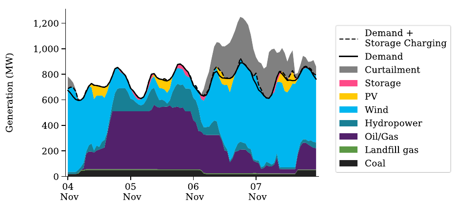
44
This report is available at no cost from the National Renewable Energy Laboratory (NREL) at www.nrel.gov/publications.
Figure 20. An example period in the 2040 Reference scenario with a rapid change in renewable
output and response from hydropower and fossil generators
7.5.1 Increased Ramping and Part-Load Operation of Thermal Plants
The increased contribution of renewables inherently reduces the generation from existing fossil
resources and changes how those resources are operated. Figure 21 isolates the response of the
fossil-fueled generators to the variation in renewable output shown in Figure 20. On the
afternoon of November 4, the wind and solar output (gray) drops continuously and the other
generators in the system must increase output, with fossil generation (orange) increasing by 388
MW in this period, increasing as much as 133 MW during 1 hour.

45
This report is available at no cost from the National Renewable Energy Laboratory (NREL) at www.nrel.gov/publications.
Figure 21. Response of Railbelt fossil fuel generators (orange) to a large reduction in wind and
solar output (gray) on November 4, 2040, in the Reference scenario
As a result of this type of operation, fossil fuel plants will spend more time varying output. Note
that Figure 21 does not show unpredictable subhourly variability that would be addressed via the
additional operating reserves assumed in this study and accounted for in the avoided cost
calculations. Figure 22 summarizes the fraction of time the Southcentral Power Project spends in
four different operational modes. (This does not include the fraction of time that the plant is
unavailable because of forced outages or for scheduled maintenance.) This plant is one the most-
efficient and lowest-cost gas-fired generators and currently operates at very high capacity factors
(about 70% in 2022).
78
In the figure, the red bar represents full output, and in the 2024
simulation, the plant spends most of the time operating in this mode. As renewable generation
increases and net load decreases, the plant spends more time operating at less than full output
and varying output between minimum and maximum, shown in the green bar. The plant also
spends a greater amount of time operating at its minimum generation point (orange bar). This
occurs when net load drops substantially but the plant must remain online to provide operating
reserves or be able to respond quickly to an increase in net load. Because we assume a 9-hour
startup time, along with a minimum down time, the plant cannot turn off unless it will not be
78
Data from EIA Form 923 for 2022.
Wind and solar
output drops by
over 570 MW
over the day
Fossil generation increases
by 300 MW over a 5-hour
period in the afternoon

46
This report is available at no cost from the National Renewable Energy Laboratory (NREL) at www.nrel.gov/publications.
needed for this multi-hour period.
79
The blue bar represents the fraction of time the plant is
turned off (not committed) during multi-hour or multiday periods of very high wind and solar
output.
Figure 22. Transition of the Southcentral combined-cycle plant from base load to load-following
and peaking operation
Figure 23 shows the weighted average capacity factor for the two Central region combined-cycle
units in the No New RE and the Reference scenarios. The actual reported value in 2022 (71%) is
shown in the blue dot.
80
The modeled capacity factors are higher, likely because of differences in
assumed outages and maintenance schedules and the assumption of an optimized dispatch across
the entire Railbelt. The capacity factors in the Reference scenario then drop significantly as their
use is offset by renewable generation.
79
As noted previously, we do not have forecast error for our wind, solar, and load data. This underestimates the
challenge of scheduling thermal plants. This is partially compensated for by the reserve requirements, particularly
the flexible ramping capacity, as well as the fuel storage requirements and the assumption that all combined-cycle
plants must always operate in full combined-cycle mode. Operation of the individual gas turbines would provide
more rapid response and a lower minimum generation level. Our assumption substantially reduces the operational
flexibility but should offset some of the limitations created by assuming perfect forecasts.
80
The plants are the George M. Sullivan Generation Plant and the Southcentral Power Project. Data for 2022
generation from EIA 923.

47
This report is available at no cost from the National Renewable Energy Laboratory (NREL) at www.nrel.gov/publications.
Figure 23. Declining capacity factor of Central region combined-cycle plants
This change in operation has important implications for fuel scheduling, plant efficiency, and
maintenance requirements. These issues and cost implications are discussed in Key Finding #6.
7.5.2 Changes in Hydropower Plant Operation
As with thermal plants, the operation of hydropower units also changes with increased
deployment of wind and solar. Because several hydropower units have storage, they are
particularly useful for managing variability and uncertainty. Figure 24 provides an example of
the response from the Bradley Lake plant during the 4-day period shown in Figure 20. In this
example, the output of Bradley Lake (green) is shown along with the Railbelt-wide net load in
yellow. During the early morning of November 4, renewable generation exceeds demand,
resulting in very little net load to be met with hydropower or fossil generation. Bradley Lake
operates at its minimum output level during this period, and the plant operates at minimum
output about 40% of the time during the entire year in the 2040 Reference scenario. The rapid
reduction in wind and solar output on this day requires Bradley Lake to increase output to
maximum over this period, then continue to vary output in response to net load—driven by
renewable output across the entire Railbelt. This kind of operation, assuming Railbelt-wide joint
dispatch, may require changes to contractual agreements or other practices to minimize the costs
of operating the system.
2022 Actual

48
This report is available at no cost from the National Renewable Energy Laboratory (NREL) at www.nrel.gov/publications.
Figure 24. Operation of the Bradley Lake hydropower plant during periods of highly variable
renewable output
7.5.3 Changes to Intertie Flow
To minimize the costs of system operation across the entire Railbelt, the scenarios assume that
both the Alaska and Kenai interties may be operated in response to the increased regional
variability of energy supplies. This means that the power flow across the intertie (including
direction of flow) may change rapidly. Figure 25 shows the same 4-day period as Figure 24,
illustrating the changes occurring on the northern part of the Railbelt. At the beginning of this
period, the supply of wind in the GVEA region (orange) exceeds its local demand, and this
excess supply of wind can be used to offset gas-fired generation in the Central region. This extra
wind energy is exported across the AK Intertie, and north to south intertie flow (black) is
represented by a positive value. However the wind is steadily decreasing during this period, and
shortly after noon it becomes economic for GVEA to import electricity, represented by a
negative flow (south to north) on the AK Intertie which operates at maximum capacity for most
of November 5. Starting on the evening of November 5, there is a rapid increase in wind, which
exceeds GVEA load producing a negative net demand (gray), so flows on the Intertie flip back to
positive values, and flow at maximum capacity for much of November 6.

49
This report is available at no cost from the National Renewable Energy Laboratory (NREL) at www.nrel.gov/publications.
Figure 25. Flow on the Alaska Intertie (black) in 2040 in the Reference scenario depends largely on
the supply of wind (orange) in the GVEA region. Positive numbers represent a flow from GVEA to
the Central region.
Figure 26 (top) shows the flow on the Alaska Intertie using a duration curve, which indicates the
number of hours per year the intertie flows are at or above a certain level. In this case, a positive
value represents flow from GVEA to the Central region. In 2024 (black), the intertie is used
primarily to import lower-cost natural gas generation into GVEA from the Central region and
reduce the need to operate more-expensive oil-fired units. The 2040 No New RE scenario (blue)
GVEA remains largely an importer, but there is some flow north to south because of the addition
of coal-fired capacity in the GVEA area that results in occasional periods where this lower
(variable cost) resource is available. In the Reference Scenario, a very large amount of wind is
built in the GVEA area due to the availability of higher quality wind, and the intertie spends
more than half the time flowing toward the Central region. For similar reasons flows on the
Kenai Intertie (bottom) are largely from HEA to Central, exporting generation from Bradley
Lake as well as substantial additional wind in the Reference scenario.

50
This report is available at no cost from the National Renewable Energy Laboratory (NREL) at www.nrel.gov/publications.
Figure 26. Regional transmission flows, where positive values represent flows from north to
Central (AK Intertie) and south to Central (Kenai Intertie)
HEA to
Central
GVEA to
Central
Central
to GVEA

51
This report is available at no cost from the National Renewable Energy Laboratory (NREL) at www.nrel.gov/publications.
7.5.4 Renewables Dispatch for Balancing Load and for Reserve Provision
Wind and solar energy have zero fuel costs, and when acquired via power purchase agreements
are often considered “must-take” resources—meaning that the utility must pay for all output
from the plant. This means that choosing to curtail renewable output reduces its economic value.
However, as costs of renewable energy fall and contribution increases, there will be greater need
to vary the output of renewable generators, dispatching the resource by reducing its output to less
than it could generate under prevailing weather conditions.
81
The need to curtail energy is shown previously in Figure 20 when during the afternoon of
November 8, the supply of renewable energy exceeds the demand for electricity across the entire
Railbelt. The output of all hydropower and fossil generators is reduced to minimum, with some
fossil generators remaining online so they can increase output during a later hour. Some of the
excess renewables are stored (shown by the demand plus storage charging line), but there is still
surplus energy that must be curtailed. During other hours, curtailment results from limited
transmission capacity. For example, on November 6, there is significant curtailment but also
large amounts of fossil generation that could have potentially been reduced. But some of the
oversupply of renewables occurs in the GVEA area, seen in Figure 25, where the net load falls
well below zero. The oversupply is greater than the transmission capacity of the AK Intertie, and
there is substantial curtailment of wind energy.
Curtailment could be reduced by increased use of storage, but using storage exclusively to avoid
curtailment has limited cost-effectiveness. Storage has the highest value when it can provide
multiple services, including provision of operating reserves. In systems without significant
renewable generation, operating reserves must respond to the potential rapid loss of conventional
generators because of failure or to the random and uncertain variations in supply. In a system
with large amounts of renewables, operating reserves must also address their variable and
uncertain nature.
Figure 27 (top) shows the total assumed (upward) operating reserve requirement in the No New
RE and Reference scenarios (black line). This is expressed in terms of GW-hrs, which is a unit of
responsive capacity available for a certain amount of time.
82
This means that 1,000 GW-hr
corresponds to having, on average, 114 MW (0.114 GW) of upward reserve capacity during each
hour of the year (8,760 total hours per year). By 2040, the Reference scenario requires, on
average, about 340 MW of available capacity to provide these reserves, which more than doubles
the reserve capacity needed on average in the No New RE scenario. At the same time, the
reduced generation from existing fossil and hydropower plants increases their availability to
81
Curtailment of renewable energy is technically easy and involves the reduction in output of generation from the
power plant. With wind, this involves mechanically changing the angle of the wind turbine rotors to reduce their
efficiency in converting wind energy to mechanical energy. In a solar plant, the power electronics are instructed to
convert less of the direct current electricity supply coming from the panels to grid power.
82
In the charts, the total reserves provided exceed the requirement. This is because during some periods, the
available spare capacity from wind and hydropower generators providing energy exceeds the requirement. For
example, if the demand for electricity is 300 MW and this is met by two 200-MW generators, there is 100 MW of
“headroom” in these generators—some of which could be used to provide reserves. We included downward reserve
requirements in the simulations but do not show these results because they are typically far less costly to provide
than upward reserves.

52
This report is available at no cost from the National Renewable Energy Laboratory (NREL) at www.nrel.gov/publications.
provide these reserves. Curtailed wind and solar also provide an increasing amount of reserves.
Wind has been used to provide regulating reserve in the United States since the early 2010s.
83
The output from the wind power plant can be increased or decreased in a controlled manner over
its available output range in less than 1 minute, while the output from solar can be controlled
over its output range in a few seconds. It is generally uneconomic to curtail wind and solar just
for provision of reserves if they could otherwise avoid fossil generation; curtailed renewable
energy must be paid for at the same rate as consumed renewable energy.
Figure 27 (bottom) shows the upward reserve requirement by type as well as the resource
providing those reserves. Contingency reserves require very rapid response and so is mostly
provided by batteries, which can respond nearly instantly. Wind and solar can also provide
frequency-responsive reserves, and all new wind turbines sold in the United States are required
to have frequency-responsive capability. However, for the purposes of this analysis, we did not
allow wind and solar to provide contingency reserves.
Figure 27. Total annual operating (upward) reserves provision by generator type (top) in the No
New RE and Reference scenarios. Total requirement is the black bar. Reserves requirement by
type for the Reference scenario is shown in the bottom. The same legend applies to all plots.
83
P. L. Denholm, Y. Sun, and T. T. Mai, 2019. An Introduction to Grid Services: Concepts, Technical
Requirements, and Provision from Wind. Golden, CO: National Renewable Energy Laboratory. NREL/PR-6A20-
73590. https:/doi.org/10.2172/1505934.

53
This report is available at no cost from the National Renewable Energy Laboratory (NREL) at www.nrel.gov/publications.
7.6 Finding #6: Cost Impacts of Addressing Variability and
Uncertainty Are Modest Relative to Savings but With Remaining
Uncertainties
All results presented in this analysis include the impact of several factors associated with
addressing variability and uncertainty, which increases the cost or reduces the net value of
renewable energy. Additional capital costs needed to support renewable integration can increase
the total cost of the renewable scenario, while variability of renewable supply can change how
the fossil fleet is operated and reduces the amount of fuel avoided.
Some of these increases in costs, including fuel storage and power plant starts, are shown in
previous results, but others—including additional operating reserves and impacts of part-load
heat rate—are “embedded” in the results and must be isolated through additional analysis.
For example, Figure 28 shows the total start costs (fuel and nonfuel costs including addition
maintenance) in the No New RE scenario (blue) and the Reference scenario (orange). By the
early 2030s, the Reference scenario incurs about $3 million per year in additional costs (which
are embedded in all results shown previously).
Figure 28. Annual fossil plant start costs are about $3 million greater per year by the early 2030s
in the Reference scenario compared to the No New RE scenario
Figure 29 summarizes the impact of all these factors, showing the annual cost of renewable
purchases plus costs associated with addressing renewable variability and uncertainty. The left
set of bars show the total costs of renewable energy purchases and integration. The bottom four
bars are the same as shown previously, including the cost of renewable purchases, spur line
costs, natural gas storage and scheduling/forecasting.

54
This report is available at no cost from the National Renewable Energy Laboratory (NREL) at www.nrel.gov/publications.
In addition to these “direct” costs, we also add the three bars associated with changes in costs
associated with system operation that result from wind and solar variability. The first is the
increased costs associated with plant stops and starts shown in Figure 29. The next is the impact
of part load heat rate, which is not necessarily a “cost” but actually a reduction in value of
avoided fuel. The deployment of renewables in the Refence Scenario decreases total natural gas
generation by about 68%, but the reduced efficiency of operation for the remaining generation
slightly decreases the value of this reduced generation. Across the entire fleet, part-load
operation reduces the value of renewables by about $2 million/year after 2030. Ascribing this as
a cost therefore is potentially misleading, since it is a reduction in value as opposed to a direct
cost, and can result in potential double counting. This is one example of how methods to
calculate “integration costs” of renewable resource is challenging and somewhat controversial.
84
A similar approach was taken to calculate the impact of additional operating reserves, which may
also include both an increase in costs (if new generation resources are required) and a reduction
in value when plants providing reserves operate less efficiently.
85
Overall, the costs of integrating wind and solar and addressing variability add about $45M/year
by 2040 (and about $435M cumulatively from 2024-2040). This can be compared to the
potential value costs avoided by this generation.
86
The difference in the total renewables cost
(left bars in Figure 29) and avoided costs (right) produces the net value, which averages $105M
from 2030 to 2040 as shown in Finding #1.
84
Milligan, M., Ela, E., Hodge, B. M., Kirby, B., Lew, D., Clark, C., DeCesaro, J., and Lynn, K. Cost-Causation and
Integration Cost Analysis for Variable Generation. United States: 2011. Web. doi:10.2172/1018105.
85
To isolate the impact of additional operating reserves because of wind and solar, we analyzed a scenario where the
additional operating reserve requirement because of new renewable capacity was not included.
86
To avoid double counting, the costs associated with embedded factors such as part-load heat rate must be added
back into the avoided fuel quantities. This is because all values for avoided fuel reported earlier already include the
impact of part-load heat rates. If we back-calculate this impact and add this as a cost to renewables, we must then
subtract this “negative benefit” from the avoided fuel.
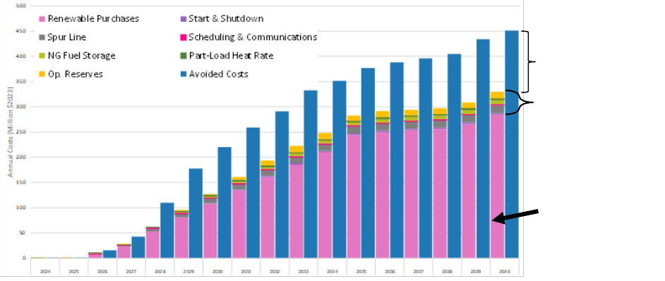
55
This report is available at no cost from the National Renewable Energy Laboratory (NREL) at www.nrel.gov/publications.
Figure 29. Annual costs ($2023) of renewable energy, including integration and addressing
resource variability, are shown in the left set of bars. These costs are included in all scenarios but
are broken out here for clarity. These increase renewable costs by about 16% compared to the
cost of only the renewable generator and interconnection. The right (blue) bars show the value of
avoided variable costs, with the difference being the net savings associated with renewable
deployment.
Although it can be difficult to determine the costs associated with integrating renewable energy,
these impacts are important not only to accurately assess the value of variable and uncertain
resources but also to consider when allocating system costs across multiple utilities. These costs
may be borne disproportionately by certain utility-owned assets, particularly those that provide
the majority of the load-following and cycling required.
There is still considerable uncertainty about these factors, particularly natural gas fuel storage.
Figure 30 shows the daily fuel requirements for all natural-gas-fueled plants in the Railbelt. In
the No New RE scenario, the fuel use largely tracks the overall seasonal load patterns, and the
range of daily natural gas fuel demand over the entire year is between 54,00 and 130,000
MMBtu. The Reference scenario always uses less gas during any given day but with larger day-
to-day variability.
Cost of renewable
purchases
($285
M
in 2040)
Cost of renewable
integration and
addressing variability
($45M in 2040)
Net savings
($
122M in 2040)

56
This report is available at no cost from the National Renewable Energy Laboratory (NREL) at www.nrel.gov/publications.
Figure 30. Daily natural gas fuel consumption in 2040
The actual impacts of this gas demand variability are difficult to assess. We add about 40 million
standard cubic feet of storage in the Reference scenario by 2040 to accommodate the increased
variability in natural gas use. The costs of this storage increase over time, reaching about $9.5
million/year in the base scenario. Additional issues related to fuel scheduling may be contractual
and are beyond the scope of this analysis. Some gas demand variability may be mitigated by
changing operational practices. The costs of these mitigation options would need to be compared
to additional flexibility in the natural gas supply.
7.7 Additional Findings
7.7.1 Potential Distributed PV Adoption Must Be Evaluated in the Context of
Incentives and Rate Structure Changes
The distributed PV (DPV) sensitivity assumes that customers adopt rooftop and other DPV based
on the schedule in Figure 41 and are responsible for all capital and O&M costs. The utility incurs
the integration-related costs associated with providing operating reserves, plant cycling, and fuel
storage. However, distribution system upgrades or incentives are not accounted for.
As a result of the additional generation on the system, the Railbelt utilities do not need to provide
as much energy. Figure 31 summarizes the change in generation mix in the DPV sensitivity,
where the added PV offsets mostly utility-procured solar but also some wind generation from

57
This report is available at no cost from the National Renewable Energy Laboratory (NREL) at www.nrel.gov/publications.
existing fossil generation. This also means that the DPV sensitivity provides a slightly higher
renewable fraction than the Reference scenario.
Figure 31. Changes in generation mix between the Reference scenario and DPV sensitivity
If the capital costs of deploying DPV are borne entirely by the consumer, this results in a
reduction in expenditures by the utility. This is shown in Figure 32 (top) as the annual reduction
in costs by category in the DPV sensitivity compared to the Reference scenario. The use of DPV
reduces costs of both utility-scale renewables (both wind and solar) and natural gas. Figure 32
(bottom) shows the effective avoided cost associated with this distributed PV, or the utility
expenditures required per unit of distributed PV generation.

58
This report is available at no cost from the National Renewable Energy Laboratory (NREL) at www.nrel.gov/publications.
Figure 32. Changes in annual costs, with the DPV sensitivity (top) showing reduction in required
utility expenditures. The avoided cost associated with the DPV sensitivity (bottom) shows the
costs utilities would have to pay for electricity to replace the DPV.
An important question is how the benefits of reduced utility expenditures compare to the actual
costs needed to achieve this scenario. These costs include potential incentives or system
upgrades required to achieve this level of deployment. Determining this would require a more
detailed analysis of existing and future rate structures, potential adoption patterns, and Alaska-
specific conditions of solar performance and distribution networks. This includes consideration
of how reduction in revenue from consumers would impact the portion of bills associated with
fixed costs of generation, transmission, and distribution, which are likely not reduced with the
use of DPV in a winter-peaking system such as Alaska.
59
This report is available at no cost from the National Renewable Energy Laboratory (NREL) at www.nrel.gov/publications.
7.7.2 The Small Increase in Costs Associated With an 80% RPS Are Largely
Because of Renewable Curtailment
Figure 10 (Section 7.1) shows that new wind and solar are substantially cheaper than the variable
cost of power plant operation, and the results of the Reference scenario show significant benefits
of deployment. However, as deployment increases (particularly as it approaches 80%), the value
of renewables drops because of a variety of factors, including the use of lower-quality wind
resources (as the best sites are used up) and increased curtailment of renewables. Curtailment
increases the cost of renewables because it represents energy that must be paid for but is not
actually used. Curtailment results from the supply-demand mismatch of renewables and demand
and limits to transmission capacity. Figure 33 illustrates this issue, showing the systemwide
dispatch during a 5-day period in the Reference scenario. The top figure shows the year 2030,
where the annual contribution of renewables reaches about 54%, but there is significant hourly
and seasonal variation in renewable contribution. During this 5-day period, we begin to see
periods when the amount of renewable supply exceeds electricity demand. Some of this extra
renewable supply can be stored, but there is still an oversupply that must be curtailed. The
bottom figure showing the same period from 2032 when annual renewable contribution has
increased to 64%. During these five days renewables have largely displaced fossil generation,
and most additional renewable generation during this period will be curtailed.

60
This report is available at no cost from the National Renewable Energy Laboratory (NREL) at www.nrel.gov/publications.
Figure 33. Curtailment occurring on a 5-day period in 2030 with annual renewable contribution of
54% (top) and 2032 (bottom) when the annual contribution of renewables has increased to 64%
Figure 34 shows the fraction of solar and wind energy curtailed as a function of renewable
energy fraction in the Reference and RPS scenarios. In all figures and results throughout this
report, renewable generation—and the fraction of generation from renewables—considers only
the usable supply. Curtailed renewables do not count towards their contribution, but this
curtailed energy must still be paid for. Curtailment rates vary regionally, with wind in GVEA
having much higher levels due to transmission constraints.

61
This report is available at no cost from the National Renewable Energy Laboratory (NREL) at www.nrel.gov/publications.
Figure 34. Annual wind and solar curtailment rate shows a dramatic increase when renewable
contribution exceeds 50%-60%
Significant curtailment does not occur until renewable contribution exceeds 50%–60%, but the
rate of curtailment increases dramatically after this point because the demand for electricity is
completely met by renewable energy in many hours of the year. As curtailment rates increase,
the effective cost of additional renewable energy increases, and each unit of renewable energy
production curtailed is unable to avoid fossil generation. This increase in cost (or decline in
value, depending on perspective) is inherently calculated by the model because it performs
hourly simulations that determine the fuel avoided by additional renewable generation. Figure 34
shows the average curtailment rates, but the incremental (marginal) curtailment rates are much
higher. For example, in the Reference scenario (with 76% renewable contribution in 2040), more
than 50% of the potential generation from additional renewable capacity (meaning capacity
added to increase the renewable contribution beyond 76%) is curtailed. This means that the
effective capacity factor of this additional resource is less than half the potential capacity factor
of an uncurtailed resource, and the effective LCOE of the usable wind generation is more than
twice the base (uncurtailed) LCOE.
87
Cost of new wind and solar installed in 2040 has fallen to
about $50/MWh (including transmission and natural gas storage), but the effective LCOE of
incremental wind and solar after curtailment is over $100/MWh (in $2023). This net cost is
higher than the avoided cost of running the remaining gas plants, so it is uneconomical to add
87
This is because the effective LCOE is equal to the annual cost divided by annual generation. If annual generation
drops by half, the effective LCOE doubles because the same amount of costs must be recovered by a smaller amount
of usable energy.

62
This report is available at no cost from the National Renewable Energy Laboratory (NREL) at www.nrel.gov/publications.
additional wind beyond about 76%, which explains why the model stops building additional
renewable capacity in the Reference scenario.
This increase in curtailment can be mitigated to some extent via storage, but the seasonal
mismatch of supply and demand limits the ability of technologies such as batteries to cost-
effectively shift supply of renewable resources—and other technologies, such as longer-duration
storage (not evaluated in this work) may be needed to address this decline in renewable value in
an 80% RPS.
7.7.3 There May Be Additional Costs or Operational Requirements To Address
the Reduced Role of Synchronous Generation and Increased Contribution
of Inverter-Based Resources
Wind, solar, and battery storage use inverters, as opposed to the synchronous generators used by
fossil and hydropower generators. Inverter-based resources (IBRs) do not have the same
characteristics as synchronous machines, including the lack of real physical inertial response and
lack of fault current provision. Alternatively, IBRs can react more rapidly than synchronous
machines to frequency deviations if programmed to do so.
88
In these simulations, we placed no restrictions on the instantaneous contribution of inverter-
based resources, and although the simulations do not reach 100% IBR contribution in part
because of the minimum generation levels on hydropower units, the levels are likely high enough
to require additional changes to maintain frequency stability, system strength, and fault current
(among other factors). We assume the extensive use of grid-forming inverters (and add
associated costs) to address some of these issues, but without further study it is not possible to
determine further changes needed or quantify possible cost impacts. However, we note that there
are several possible pathways to allow for such high levels of IBRs. In the shortest term, this
could include changing unit commitment and dispatch to ensure that a certain amount of
synchronous generation remains online. This has been performed in locations including Texas
and Ireland. The limitation of this approach is the increase in costs associated with keeping
thermal plants operating at minimum generation levels and associated curtailment. This is
typically considered a temporary measure as grid operators deploy the necessary technologies to
allow for greater instantaneous IBR contribution.
There are a variety of approaches to provide the necessary grid services, but one of the more
commonly discussed is the use of synchronous condensers. Synchronous condensers would spin
up during periods of very high IBR contribution, particularly if grid-forming inverters are unable
to provide all the necessary services to maintain frequency stability, system strength, or fault
current. This approach is likely more expensive compared to approaches based on power
electronics but has the advantage of being well understood and provides a “bookend” for a
possible upper bound of costs that maintains a synchronous-machine-based grid.
The construction of dedicated new synchronous condensers can be compared to the savings
calculated in this work. The average annual savings from 2030 to 2040 is about $105M/year
88
Denholm, P., Y. Sun, and T. Mai. 2019. An Introduction to Grid Services: Concepts, Technical Requirements, and
Provision from Wind. Golden, CO: National Renewable Energy Laboratory. NREL/TP-6A20-72578.

63
This report is available at no cost from the National Renewable Energy Laboratory (NREL) at www.nrel.gov/publications.
($2023). The annual cost of financing and operating 250 MW of new synchronous condensers at
$300/kW would be about $10M/year.
89
This would reduce the annual benefits of renewables by
about 10% to about $95M/year over the 2030 to 2040 time frame. Further analysis is required to
determine the least-cost approach to maintain grid services. For example, in addition to power-
electronics-based alternatives, existing plants may potentially be retrofitted to operate as
synchronous condensers, reducing costs.
90
7.7.4 Replacing Retiring Renewables Beyond 2040 Should Be Less Expensive
Than Additional Natural Gas Generation
This analysis extends only to 2040. Beyond this date, there will be eventual retirements of wind
and solar projects, although we assume that this will not be required at significant scale before
about 2050. With the expiration of the federal tax credits, the cost of building new wind and
solar increases. Looking beyond 2040 is highly speculative, but with the assumed cost
trajectories for natural gas, wind, and solar, adding new wind and solar after 2040 will still be
less expensive than burning natural gas. Removing all tax credits, the projected LCOE in 2041
(in $2023) for wind with a capacity factor of at least 33% would be less than $80/MWh, and the
LCOE of solar would be less than $70/MWh. The fuel-related costs of running existing natural
gas plants would be more than $90/MWh, so wind and solar without tax incentives will be less
than the cost of generation from gas. The cost of new wind and solar does not consider the
potential replacement of natural gas storage infrastructure and some other costs of integration nor
does it consider the opportunity to repower existing plants with new equipment, avoiding many
of the site development costs.
89
This would maintain over 400 MW of synchronous machine capacity throughout the Railbelt when including
existing hydropower capacity. In addition to capital costs, this value assumes a $15/kW-year fixed O&M cost.
Synchronous condensers also require operating costs including energy used to drive the machine. Most of the
operation of the synchronous condensers will occur during periods of significant curtailment; therefore, unused
renewable energy will be used for a large fraction of this energy.
90
An example of an LM6000 gas turbine retrofit is discussed here:
https://www.turbomachinerymag.com/view/spinning-res
erve-commonwealth-chesapeake-gives-lm6000s-double-
duty.
64
This report is available at no cost from the National Renewable Energy Laboratory (NREL) at www.nrel.gov/publications.
8 Conclusions
The projected prices for natural gas in the Railbelt region result in costs of generation from
existing natural gas plants in the range of $70 to $80/MWh by the end of this decade, with
considerable price uncertainty and potential volatility. With projected declines in the cost of
wind and solar, along with the extension of federal tax credits, these resources can offer
generation with stable, long-term contracts at less than the projected cost of natural gas
generation in this time frame. Based on the assumptions used in this analysis, achieving more
than a 75% contribution of renewables toward Railbelt electricity by 2040 appears to be the
least-cost option. This includes the impact of additional costs associated with natural gas storage
and other requirements to address the variability and uncertainty of wind and solar generation.
Moving to an 80% RPS slightly decreases the overall benefit of renewables deployment because
the mismatch of renewable supply and electricity demand limits the ability of renewables to
displace the remaining fossil generation. However, based on the modeling assumptions used, the
cost difference between the least-cost scenario and the RPS scenario is very small—especially
compared to the impact of the uncertainty range of future prices of renewables and natural gas.
There are also several other significant uncertainties around the scenarios evaluated in this work
that could impact this result, including the potential load growth driven by EVs and electric
heating.
Additional modeling will be required to validate the findings of this work, particularly in the
changes to operation needed. This includes additional modeling to ensure system stability during
periods when inverter-based wind, solar, and storage provide most of the energy as well as
required hardware costs to address the lack of synchronous generators during these periods. In
addition, the following items would allow for a more comprehensive assessment of renewable
energy options in the Railbelt:
• Improved solar data. The impact of solar variability could not be accurately assessed in this
modeling because of a lack of time-synchronized solar data across large regions.
• Analysis of wind and solar forecast error and sub-hourly variability.
• Impact of changing weather patterns.
• Modeling transmission options for the Alaska Intertie upgrades and assessing transmission
alternatives.
• Deeper assessment of distributed resources such as solar, wind, and storage, including
impacts on utility revenue and cost recovery.
• Detailed analysis of new hydro options.
• Consideration of capital costs of natural gas infrastructure including required storage and
deliverability under uncertainty.
65
This report is available at no cost from the National Renewable Energy Laboratory (NREL) at www.nrel.gov/publications.
Appendix A. Capacity- and Energy-Related Terms
Capacity (also “nameplate capacity” or “peak capacity”) generally refers to the rated output of a
power plant when operating at maximum output. The capacity of individual power plants is
typically measured in kilowatts (kW) or megawatts (MW). The cumulative capacity of systems is
often measured in gigawatts (GW) or terawatts (TW). Capacity of power plants is typically
measured by their net AC rating, and we use this standard in this report.
Energy, in this report, refers to electricity generated and used for lighting, appliances, etc. It is
typically measured in kilowatt-hours (kWh) and represents one kW of power used for an hour.
Capacity factor (%) is a measure of how much energy is produced by a plant compared to its
maximum output. It is calculated by dividing the total energy produced during some period of
time by the amount of energy it would have produced if it ran at full output over that period.
Capacity credit is a measure of the contribution of a power plant to resource adequacy, meaning
the ability of a system to reliably meet demand during all hours of the year. It is measured in
terms of either capacity (kW, MW) or the fraction of its nameplate capacity (%) and indicates the
amount or portion of the nameplate capacity that is reliably available to meet load during times
of highest system demand—typically the highest net load hours of the year.

66
This report is available at no cost from the National Renewable Energy Laboratory (NREL) at www.nrel.gov/publications.
Appendix B. Base Modeling Assumptions
B.1 Utility-Owned Fossil Generators
Table B-1 summarizes data for existing utility-owned assets using data submitted by each utility
to the Energy Information Administration (EIA) on Form 860m.
91
Based on feedback including
proprietary data from individual utilities, there are some small differences between these data
and data actually used in the model. Utility names and plant names are abbreviated for brevity.
Table B-1. Existing Railbelt Fossil Fuel Generators (data as reported to EIA)
Utility
Name
Plant Name
Gen. ID
Nameplate
Cap. (MW)
Net
Summer
Cap.
(MW)
Net
Winter
Cap.
(MW)
Type
Operating
Year
Status
Chugach
Hank Nikkels
3R
48.9
29.3
32.9
NGCT
2007
OP
Chugach
Hank Nikkels
P1 BS
2.0
2.0
2.0
Oil ICE
2012
OP
Chugach
George M Sullivan
7
102.6
102.6
81.8
NGCT
1979
OP
Chugach
George M Sullivan
CC
151.7
129.0
129.0
NGCC
2017
OP
Chugach
George M Sullivan
GT8
92.6
77.7
86.5
NGCT
1984
SB
Chugach
Southcentral
CC
203.9
169.7
203.4
NGCC
2013
OP
Chugach
Beluga
1
16.0
18.9
19.6
NGCT
1968
SB
Chugach
Beluga
3
59.1
58.0
64.8
NGCT
1972
SB
Chugach
Beluga
5
68.3
61.4
68.7
NGCT
1975
SB
Chugach
Beluga
7
76.5
70.6
80.1
NGCT
1978
SB
Seward
Seward
3
2.5
2.5
2.5
Oil ICE
1975
OP
Seward
Seward
4
2.5
2.5
2.5
Oil ICE
1986
OP
Seward
Seward
5
2.5
2.5
2.5
Oil ICE
1985
OP
Seward
Seward
6
2.8
2.8
2.8
Oil ICE
2000
OP
Seward
Seward
N1/N2
5.3
5.3
5.6
Oil ICE
2010
OP
GVEA
Healy
1
28.0
25.0
25.0
Coal
1967
OP
GVEA
Healy
2
62.0
50.0
50.0
Coal
1998
OP
GVEA
North Pole
1
60.5
44.0
60.0
Oil CT
1976
OP
GVEA
North Pole
2
60.5
50.0
64.0
Oil CT
1977
OP
GVEA
North Pole
GT3/STG1
60.0
51.0
65.0
Oil CC
2007
OP
GVEA
Fairbanks
GT1
18.4
15.5
17.7
Oil CT
1971
OP
GVEA
Fairbanks
GT2
18.4
15.0
17.7
Oil CT
1972
OP
GVEA
Delta Power
6
23.1
23.1
26.0
Oil CT
1976
SB
HEA
Seldovia
5
1.2
1.2
1.2
Oil ICE
2004
OP
HEA
Seldovia
7
1.0
1.0
1.0
Oil ICE
2017
OP
HEA
Bernice Lake
2
20.7
17.0
19.0
NGCT
1971
OP
91
https://www.eia.gov/electricity/data/eia860m/.

67
This report is available at no cost from the National Renewable Energy Laboratory (NREL) at www.nrel.gov/publications.
Utility
Name
Plant Name
Gen. ID
Nameplate
Cap. (MW)
Net
Summer
Cap.
(MW)
Net
Winter
Cap.
(MW)
Type
Operating
Year
Status
Utility
Name
Plant Name
Gen. ID
Nameplate
Cap. (MW)
Net
Summer
Cap.
(MW)
Net
Winter
Cap.
(MW)
Type
Operating
Year
Status
HEA
Bernice Lake
3
28.8
22.9
26.0
NGCT
1978
OP
HEA
Bernice Lake
4
27.2
22.5
26.0
NGCT
1981
OP
HEA
Nikiski
GT1
40.8
37.9
42.0
NGCC
1986
OP
HEA
Nikiski
ST1
40.0
38.0
40.0
NGCC
2013
OP
HEA
Soldotna
1
50.0
44.0
49.0
NGCT
2014
OP
MEA
Eklutna Gen. Station
01-10
171
165
165
NG ICE
2015
OP
Table B-2 provides the average heat rate as reported to EIA
92
in 2022, for plants that produced at
least 70 GWh in 2022. These plants provided about 80% of Railbelt generation and 94% of fossil
generation in 2022.
Table B-2. Average Heat Rate for Major Fossil Fuel Generators (producing at least 70 GWh in 2022)
Utility
Name
Plant Name
Gen. ID
Nameplate
Cap. (MW)
Type
2022
Reported
Heat
Rate
2022
Reported
Generation
(GWh)
Chugach
George M
Sullivan
CC
151.7
NGCC
7,920
872
Chugach
Southcentral
CC
203.9
NGCC
7,650
1,151
GVEA
Healy
1/2
90
Coal
13,680
405
GVEA
North Pole Gas
Turbine
1/2
121
Oil CT
11,650
71
GVEA
North Pole
Combined Cycle
GT3/STG1
60.0
Oil CC
7,660
354
HEA
Nikiski Combined
Cycle
GT1
81
NGCC
8,950
432
MEA
Eklutna Gen.
Station
01-10
171
NG ICE
8,730
532
B.2 Heat Rate and Start Cost Modeling
All generators of significant size are modeled with a heat rate curve to capture the potential
decrease in efficiency associated with increased cycling operation. Heat rate values are derived
from utility data and public sources.
93
Figure 35 provides an example of the simplified heat rate
curve used for the Southcentral combined-cycle (CC) unit in Alaska, which we show as a
92
https://www.eia.gov/electricity/data/eia923/.
93
For example, for Chugach, we used the “2021 Heat Rate Analysis Report” that includes heat rate curves for its
thermal fleet.

68
This report is available at no cost from the National Renewable Energy Laboratory (NREL) at www.nrel.gov/publications.
function of full output.
94
We do not include the impact of part-load operation on very small
plants (<10 MW), especially because most of those plants rarely run.
Figure 35. Example simplified heat rate curve for the Southcentral combined-cycle generator
Start costs include both the start fuel requirements and nonfuel costs. Data were derived from the
utilities or from previous National Renewable Energy Laboratory (NREL) studies where utility
data were not available.
95
For CC plants, we assume that all starts require operation in full CC
mode (all gas turbines) and not the operation of individual combustion turbines without the
steam turbine. This is a conservative estimate that reduces the flexibility of the system.
B.3 Treatment of CHP Plants and Other Nonutility-Owned Generators
There are about 100 MW of nonutility fossil-fueled generation facilities in the Railbelt and
connected to the Railbelt grid. These are largely combined heat and power (CHP) plants serving
military bases, industrial customers, and the University of Alaska-Fairbanks (UAF). These plants
largely serve native loads, and load data from the utilities do not include the load served by these
CHP plants. Railbelt utilities make no significant purchases of energy from these resources
except Aurora and UAF. Aurora is a coal-fired plant that provides combined heat and power to
Fairbanks, and because it provides heating, is modeled as a must-run unit throughout the winter
(January through April; October through December). During this period, Aurora is committed
and can vary its output between 19 MW and 22 MW. During the summer, it is treated as a
utility-dispatched resource.
96
Based on data from Golden Valley Electric Association (GVEA),
we also assume that 4 MW of UAF (coal generation) capacity is utility-dispatched.
B.4 Hydropower
Existing hydropower plants are listed in Table B-3.
94
We use a “piecewise linear” approximation of the polynomial heat rate curve.
95
WWSIS-2.
96
This may require changes to long-term purchase contracts.
7
7.25
7.5
7.75
8
8.25
8.5
8.75
9
0 25 50 75 100 125 150 175
200
Heat Rate (BTU/kWh)
Power (MW)

69
This report is available at no cost from the National Renewable Energy Laboratory (NREL) at www.nrel.gov/publications.
Table B-3. Existing Railbelt Hydropower Plants
Name Power Minimum
Generation
Level
Notes
Bradley Lake 1 60
6
EIA lists as 63 for all three
ratings
Bradley Lake 2 60 6 EIA lists as 63
Cooper Lake 1 9.7 6.5
Cooper Lake 2 9.7 6.5
Eklutna Hydro 1 20 3.0 EIA lists as 22
Eklutna Hydro 2 20 3.0 EIA lists as 22
Plants are dispatched based on maximum and minimum outputs, and we assumed a monthly
average water supply for existing hydropower generators (Table B-4). Monthly water supply for
existing hydropower generators was obtained from EIA-923 and from the Alaska Energy
Authority (AEA).
Table B-4. Monthly Water Budget for Existing Railbelt Hydropower Plants
Month
Monthly Water Availability (GWh)
Bradley Lake
Units 1 and 2
Cooper Lake
Units 1 and 2
Eklutna Hydro
Units 1 and 2
Jan 19.83 1.85 7.1
Feb 16.5 1.54 5.91
Mar 15.82 1.47 5.67
Apr 13.96 1.3 5
May 17.29 1.61 6.19
Jun 18.62 1.73 6.67
Jul 16.58 1.54 5.94
Aug 15.64 1.46 5.6
Sep 12.83 1.19 4.59
Oct 13.17 1.23 4.71
Nov 15.43 1.44 5.52
Dec 19.83 1.84 7.1
B.5 Other Existing Resources
Table B-5 lists other generation resources in operation in the Railbelt. Location of existing wind
is shown in Figure 37.

70
This report is available at no cost from the National Renewable Energy Laboratory (NREL) at www.nrel.gov/publications.
Table B-5. Existing Railbelt Renewable Generators
Name Nameplate
Capacity (MW)
Type
Fire Island Wind 18 Wind
Eva Creek Wind 24.6 Wind
Delta Wind Farm 1.9 Wind
JBER 11.5 LFG
Willow Solar 1 Solar
Houston Solar 6 (8.5 DC Rating) Solar
B.6 Electric Vehicle Adoption
For the Reference scenario, we used the lowest growth level, from the “AEA continued”
forecast, shown in Figure 36, which results in about 110,000 vehicles (about 20% of all vehicles
in the Railbelt) in 2040 (left y-axis). Annual customer demand at the meter is shown in the right
axis (before transmission and distribution [T&D] losses). Demand profiles (including additional
T&D losses) for 2040 are shown in Figure 36 (bottom) and vary hourly and seasonally, based on
driving patterns and demonstrating the impact of cold-weather performance.
97
For other years,
the profiles are scaled proportionally to the number of vehicles shown in the top of the figure.
The loads were allocated to the three zones based on Alaska Center for Energy and Power
(ACEP) data.
98
We assume that the charging demand profiles are completely inflexible.
97
The ACEP study uses typical weather year data, which do not match the 2018 weather year used in our study,
which could over- or underestimate the actual impacts of vehicle charging during any given hour or day. The most
significant impact in our use of these mismatched data could be underestimating the load on a peak demand day,
resulting in an overestimation of resource adequacy. Fortunately, the demand in the ACEP data on the day of our
studies’ peak demand day is close to the annual peak demand in the ACEP data, minimizing this concern.
98
Cicilio, P.; Francisco, A.; Morelli, C.; Wilber, M.; Pike, C.; VanderMeer, J.; Colt, S.; Pride, D.; Helder, N.K. Load,
Electrification Adoption, and Behind-the-Meter Solar Forecasts for Alaska’s Railbelt Transmission System. Energies
2023, 16, 6117. https://doi.org/10.3390/en16176117

71
This report is available at no cost from the National Renewable Energy Laboratory (NREL) at www.nrel.gov/publications.
Figure 36. EV adoptions (top) and Reference scenario charging profiles in 2040 (bottom)
B.7 Operating Reserves
Table B-6. details the assumptions of operating reserves as modeled. Unless otherwise noted, the
reserve product is provided for each zone individually, and reserves are not shared between
zones.
The additional reserve requirement for renewable energy was based on the maximum 1-hour
ramp as a fraction of generation, equal to about 60% for wind. We assume that this entire 1-hour
ramp must be served by operating reserves split between a fast component (regulation) and a
slow component (flexibility).
0
100
200
300
400
500
600
700
800
0
20,000
40,000
60,000
80,000
100,000
120,000
2024 2026 2028 2030 2032 2034 2036 2038 2040
Additional Load (GWh)
Number of Electric Vehicles
0
50
100
150
200
250
300
12:00 AM 6:00 AM 12:00 PM 6:00 PM 12:00 AM
Net EV Load Including T&D Losses (MW)
Maximum EV Load Day
Average Day
Minimum EV Load Day

72
This report is available at no cost from the National Renewable Energy Laboratory (NREL) at www.nrel.gov/publications.
Table B-6. Summary of Operating Reserve Modeling
Parameter Assumption
Contingency 80 MW for the entire Railbelt. Provided primarily with battery energy storage
systems, but some can be met using synchronized generators with a sufficiently fast
response rate (full response in 60 seconds).
Regulation 2% of load in Homer Electric Association (HEA) and Central. 5% of load in GVEA
based on utility feedback. Regulation for wind and solar is 20% of combined output
in each hour. Must be provided by synchronized generators or batteries with a 10-
minute response. Requirement is symmetric in both directions, meaning that the
same amount of both upward and downward reserves is required in all time periods.
Flexibility
40% of wind plus 10% of solar output (including distributed photovoltaics [DPV]).
Must be provided by synchronized generators or batteries with a 30-minute
response requirement. Requirement is symmetric in both directions.
Fossil/hydro
eligibility
All fossil and hydro plants can provide all reserves, limited by ramp rate and
operational status, including online status (for synchronized reserves) and available
headroom at current dispatch point.
Additional
subhourly
cycling costs
of fossil units
We assign a cost of $4.5/MWh for units providing operating reserves to represent
additional subhourly response.
99
This value is in addition to the impacts of additional
starts and part-load (steady-state) operation that result from additional operating
reserves; these are calculated separately.
Renewable
eligibility
Wind and PV can provide regulation and flexibility, but not contingency, reserves
after 2024. This is performed by curtailing the output of the plant.
100
DPV cannot
provide reserves.
Reserve
sharing
across zones
Not allowed, except for contingency reserves.
We did allow for occasional reserve shortages, particularly because these conditions were
already experiencing failures of the largest single system component, which sets the maximum
reserve requirement. We assume a cost of unserved operating reserves (violation of reserve
shortage) equal to $10,000/MW-h.
101
99
Value based on Hummon, M., P. Denholm, J. Jorgenson, D. Palchak, B. Kirby, and O. Ma. 2013. Fundamental
Drivers of the Cost and Price of Operating Reserves. Golden, CO: National Renewable Energy Laboratory.
NREL/TP-6A20-58465.
100
This is already common practice in several regions, most notably in Texas. Milligan, M., B. Frew, B. Kirby, M.
Schuerger, K. Clark, D. Lew, P. Denholm, B. Zavadil, M. O'Malley, and B. Tsuchida. 2015. “Alternatives No More:
Wind and Solar Power Are Mainstays of a Clean, Reliable, Affordable Grid.” IEEE Power and Energy Magazine
13(6): 78–87. (See also https://www.nrel.gov/docs/fy19osti/73866.pdf)
101
This is the cost of 1 MW of capacity unavailable for reserves in 1 hour. Therefore, this is a unit of capacity over
time, not energy. This is a soft constraint to allow the model to solve in challenging time periods.

73
This report is available at no cost from the National Renewable Energy Laboratory (NREL) at www.nrel.gov/publications.
Appendix C. Generator Cost and Performance
Assumptions for New Resources
Summary tables of costs for each technology are provided in Appendix 0, with a description in
the following subsections.
C.1 Land-Based Wind
We obtained simulated hourly wind production data for 38 sites with a total of about 2.9 GW of
capacity using the 2018 weather year. Wind production data are simulated from ERA5 wind
reanalysis data from 2000 to 2020 at 100 m, sped up using annual average wind speeds from
UL’s 200-m resolution downscaled wind resource models that consider terrain and other factors.
A power curve from the GE 3.4-MW/140-m turbine at hub heights of 100 m and 120 m was
applied to estimate production. Total losses of 17% are included (electrical losses, turbulence,
wake losses, downtime, cold weather package energy consumption).
102
Total resource
availability was based on land ownership and other exclusions, assuming a packing density of
wind of 3 MW/km
2
.
We process the native wind speed data into inputs for the capacity expansion model as follows.
This processing is all performed using NREL’s renewable energy potential (reV) tool.
103
First,
we apply a turbine power curve to the wind resource data (as mentioned previously) to produce
hourly capacity factor profiles at each 4-km grid cell. These cells are then masked with the
exclusion layer (shown in Figure 37) to eliminate land ineligible for wind turbine development.
The identified sites have a capacity factor range of 31% to 44% with a weighted average of about
36%.
102
Using NREL’s renewable energy potential (reV) tool with NASA data for the year 2018.
103
Maclaurin, Galen, Nick Grue, Anthony Lopez, Donna Heimiller, Michael Rossol, Grant Buster, and Travis
Williams. 2019. The Renewable Energy Potential (reV) Model: A Geospatial Platform for Technical Potential and
Supply Curve Modeling. Golden, CO: National Renewable Energy Laboratory. NREL/TP-6A20-73067.
https://www.nrel.gov/docs/fy19osti/73067.pdf.

74
This report is available at no cost from the National Renewable Energy Laboratory (NREL) at www.nrel.gov/publications.
Figure 37. Railbelt wind resource and location of wind site evaluated

75
This report is available at no cost from the National Renewable Energy Laboratory (NREL) at www.nrel.gov/publications.
Using an algorithm that optimizes turbine spacing in the resulting masked cells, we assign each
cell a maximum technical potential of wind capacity in MW. Next, we determine the
interconnection cost of each of these hypothetical wind farms by identifying the least-cost spur
line to connect it to the existing transmission network. This spur line cost is added to the base
capital cost of the wind plant. Spur line costs are estimated using the distance from the center of
the wind farm to the local transmission network, assuming a blended average distance-based spur
line cost of $11/kW-km ($17.7/kW-mile). This assumes a lower voltage (69-kV) interconnection
for smaller plants (<100 MW) using a single circuit, or a higher voltage (138-kV) double-circuit
line for larger plants.
104
We assume that the cost of the spur line is eligible for the ITC and
financed with the same terms as the wind plant.
The interconnection costs of each grid cell, combined with their technical wind potential, makes
up a supply curve. This, along with the representative hourly capacity factor profiles, is used by
the capacity expansion model. The model may then choose between various locations
considering the potential trade-off between performance and distance.
104
Value based on discussions with various stakeholders.
76
This report is available at no cost from the National Renewable Energy Laboratory (NREL) at www.nrel.gov/publications.
Table C-1. Location and Performance of Available Wind Sites Evaluated
Potential
Capacity (MW)
Lat.
Long.
Zone
Capacity
Factor
Spur Line
Distance (km)
Spur Line Cost
Per KW ($)
195
63.974
-148.406
GVEA
41.2%
36.4
400
192
64.093
-148.858
GVEA
35.3%
8.3
92
185
64.005
-149.346
GVEA
34.5%
1.0
11
182
63.99
-148.876
GVEA
36.9%
3.0
33
177
63.982
-148.641
GVEA
34.5%
33.6
369
142
64.505
-148.784
GVEA
32.6%
2.1
23
130
64.196
-148.839
GVEA
32.3%
3.8
42
113
60.028
-151.154
Homer
32.7%
5.3
58
113
63.8
-149.379
GVEA
34.9%
26.1
287
102
64.314
-149.296
GVEA
33.0%
2.1
23
97
64.101
-149.094
GVEA
34.4%
12.0
131
90
63.887
-148.894
GVEA
36.6%
3.3
36
85
63.571
-148.716
GVEA
41.3%
53.3
586
74
63.879
-148.66
GVEA
38.0%
21.0
231
71
63.792
-149.146
GVEA
36.6%
4.3
48
64
63.959
-145.805
GVEA
31.1%
8.4
92
63
61.119
-149.553
Central
35.8%
13.7
150
62
61.112
-149.339
Central
34.3%
20.3
224
61
64.599
-148.525
GVEA
33.1%
2.2
24
50
60.542
-151.109
Homer
33.6%
1.0
11
49
61.061
-151.276
Central
39.8%
29.6
325
47
59.731
-151.797
Homer
33.5%
1.8
20
45
60.649
-151.311
Homer
37.3%
0.7
8
45
64.417
-149.279
GVEA
32.7%
1.3
15
41
63.563
-148.484
GVEA
39.0%
82.6
909
40
60.752
-151.303
Homer
37.5%
10.4
115
36
59.937
-151.783
Homer
34.7%
4.9
54
33
61.065
-151.49
Central
40.3%
44.2
486
32
59.812
-150.76
Homer
43.7%
34.1
375
32
59.71
-150.77
Homer
38.7%
35.0
385
29
60.547
-151.32
Homer
35.9%
2.8
30
28
63.785
-148.912
GVEA
42.2%
8.9
98
25
61.017
-149.567
Central
33.2%
3.8
42
24
61.01
-149.354
Central
35.5%
5.8
64
23
61.242
-150.183
Central
38.1%
8.7
96
20
61.023
-149.781
Central
35.6%
20.5
225
Cost estimates use the 2023 ATB using the “technology 3” category, which assumes a 3.3-MW
turbine with a 148-meter rotor diameter and a 100-meter hub height, designed for a typical

77
This report is available at no cost from the National Renewable Energy Laboratory (NREL) at www.nrel.gov/publications.
capacity factor of about 33%.
105
The ATB data assume a 200-MW wind plant while the largest
individual wind plant in our data set is less than that. The reduced economy of scale benefits are
captured in the Alaska multiplier, which assumes that even in a mature market, the cost of wind
in Alaska is 60% higher than the ATB assumptions.
Figure 38 shows the estimated LCOE (or fixed PPA contract price) across a range of capacity
factors, before the addition of transmission interconnection costs or fuel storage costs. The
values in Figure 38 (which vary across the sites according to actual resource quality and
interconnection costs) represent the cost in the initial year of operation, which are constant in real
dollars ($2023) but would escalate at 2.5% per year in nominal dollars. The model generally
adds resources with this range of capacity factors, with a fleet average capacity factor of 35.9%
in the Reference scenario. For comparison, we also show average PPA price for contracts in the
Lower 48 signed from 2019 to 2023, adjusted to $2023.
106
The dot is the capacity weighted
average, while the bar shows the range for the 80
th
percentile of contracts in the data set.
Figure 38. Assumed LCOE/PPA price projections for utility-scale wind operating with an average)
(not including transmission). The PPA price is fixed (in real $2023) for 25 years from the year of
installation, which corresponds to an escalation at the rate of inflation in nominal dollars.
Wind is assumed to be fully dispatchable (up to the output reflecting wind conditions at any
given time) but acts as a financial “must-take” resource if obtained by a PPA. Based on the
contribution of wind during peak demand periods, we assume a capacity credit (contribution of
wind toward resource adequacy) equal to 10% of nameplate.
No new wind is allowed before the end of 2026. Starting in 2027, we assume that no more than
150 MW of wind can be completed per year.
105
https://atb.nrel.gov/electricity/2023/land-based_wind.
106
https://emp.lbl.gov/wind-power-purchase-agreement-ppa-prices.
$0
$10
$20
$30
$40
$50
$60
$70
$80
2022 2024 2026 2028
2030
2032 2034 2036 2038 2040
Wind LCOE/PPA Price (2023 $/MWh)
Year of Project Completion
AK 34% CF
AK 37% CF
AK 40% CF
Avg 2019-2022 Lwr 48 (all capacity factors)

78
This report is available at no cost from the National Renewable Energy Laboratory (NREL) at www.nrel.gov/publications.
C.2 Offshore Wind
We assume that offshore wind may be deployed starting in 2030. We did not use ATB values for
cost and performance; instead, we used data from a pending NREL study to be released in
2024.
107
Figure 39 summarizes assumed capital cost (top) and levelized cost of energy (bottom)
values for fixed-base and floating offshore wind deployed in the Cook Inlet. Costs include the
interconnection to a point near Homer. Estimated capacity factors are in the range of 50% to
52%, which is significantly higher than land-based values. However, the overall cost of energy is
significantly higher than land-based wind, and offshore wind was not deployed in the scenarios
evaluated.
Figure 39. CapEx projections for offshore wind (top) and LCOE/PPA price projections assuming a
51% capacity factor (bottom). Cost assumes underwater transmission line connecting to the HEA
system near Homer. The PPA price is fixed for 25 years from the year of installation.
107
Tentative title: Feasibility Study for Renewable Energy Technologies in Alaskan Offshore Waters.
$0
$1,000
$2,000
$3,000
$4,000
$5,000
$6,000
$7,000
2030 2032 2034 2036 2038 2040
Offshore wind Overnight Capital Cost
($/kW)
Year
AK floating AK Fixed
Lwr 48 Fixed class 4
Lwr 48 Floating class 11
$0
$10
$20
$30
$40
$50
$60
$70
$80
$90
$100
2030 2032 2034 2036 2038 2040
Offshore Wind LCOE/PPA Price ($/MWh)
Year
Floating
Fixed

79
This report is available at no cost from the National Renewable Energy Laboratory (NREL) at www.nrel.gov/publications.
C.3 Solar (PV)
We used solar profiles generated for four locations in Alaska using both tracking and fixed-tilt
systems, assuming a 1.5 DC/AC ratio.
108
PV packing density in terms of MW of DC module
capacity (MW/km
2
) is 32 MW/km
2
.
These data sets use older resource data that are not time-synchronized with our meteorological
year of 2018 because there were no alternative data available above latitude 60°N in the time
frame of the study. The lack of time-synchronized data for PV is generally not desirable because
it can lead to over- or underestimates of PV output during summer peak demand periods.
However, the lack of strong summer peaks in Alaska mitigates this data limitation. Because
Alaska is a winter-peaking system, the contribution of solar during the peak is typically
extremely low, and we therefore assume zero contribution of PV toward resource adequacy. We
assume that PV acts only as an “energy saver” and does not by itself reduce the need for firm
generation resources.
As with wind, solar is assumed to be fully dispatchable (up to the output reflecting weather
conditions at any given time) but acts as a financial “must-take” resource. New solar cannot be
completed before 2025. Assumed growth caps for solar limit deployment to 25 MW/year from
2025 to 2026, increasing to 100 MW/year in 2027. We assume that solar is deployed close to
existing transmission, and requires a relatively small spur line, which we assume adds $22/kW
and is assumed to be eligible for the 40% ITC.
C.4 Rooftop and Distributed Solar
Figure 41 summarizes the assumed adoption rate in the DPV sensitivity using the most
conservative ACEP projections.
109
Rooftop PV production is treated as a reduction in load, and
we assume that it cannot be dispatched by the utility. PV profiles are multiplied by 1.057 to
account for avoided T&D losses because generation is at (or very close) to the point of use.
Deployment of a significant amount of rooftop PV will require utilities to have “visibility” into
the amount deployed for planning and operations. As with utility-scale solar, distributed solar is
assigned zero capacity credit toward resource adequacy and requires additional operating
reserves and fuel storage to address additional uncertainty. In this sensitivity, we assume that the
adoption occurs both in the Reference and RPS scenarios and therefore has no impact on the
relative costs of the RPS. This sensitivity allows for estimates of potential avoided costs and can
then be compared to alternative portfolios.
108
https://pvwatts.nrel.gov/.
109
Cicilio, P.; Francisco, A.; Morelli, C.; Wilber, M.; Pike, C.; VanderMeer, J.; Colt, S.; Pride, D.; Helder, N.K. Load,
Electrification Adoption, and Behind-the-Meter Solar Forecasts for Alaska’s Railbelt Transmission System. Energies
2023, 16, 6117. https://doi.org/10.3390/en16176117

80
This report is available at no cost from the National Renewable Energy Laboratory (NREL) at www.nrel.gov/publications.
Figure 40. Assumed distributed/rooftop PV adoption in the DPV sensitivity
C.5 Geothermal
We assume that up to 100 MW (in 50-MW blocks) of geothermal energy (Binary Hydrothermal)
could be completed beginning in 2034 at Mt. Spurr.
110
Figure 41 shows the capital cost (top) and
LCOE (bottom) for new geothermal, which could represent a PPA price of a fixed 30-year
contract. The figure does not include the additional cost of a 73-km transmission line required to
connect the Mt. Spurr site to the meshed transmission network near Port Mackenzie. For this
cost, we use the same assumptions as wind spur lines. Geothermal is modeled as a dispatchable
resource with zero-variable cost.
111
However, if acquired via PPA, curtailed geothermal energy
must still be paid for. We do not require additional fuel storage or increased operating reserve
provisions because of any geothermal plant builds. Geothermal plants are assumed to have the
same resource adequacy contribution as fossil-fueled generators.
110
This estimate was derived from conversations with Cyrq Energy. For more information, see this report: WH
Pacific. 2013. Renewable Energy in Alaska. Golden, CO: National Renewable Energy Laboratory. NREL/SR-7A40-
47176. https://www.nrel.gov/docs/fy13osti/47176.pdf
.
111
There is a small variable cost, which is captured in the fixed O&M for the purposes of modeling, assuming
baseload generation with 80% capacity factor.
0
50
100
150
200
250
2024 2026 2028 2030 2032 2034 2036 2038 2040
Rooftop PV Installed (MW)
Total
Central
GVEA
HEA

81
This report is available at no cost from the National Renewable Energy Laboratory (NREL) at www.nrel.gov/publications.
Figure 41. Assumed geothermal capital cost (top) and LCOE (bottom)
Figure 42 shows the location of Mt. Spurr as well as other geothermal resources that could be
used for heating and other applications.
$0
$1,000
$2,000
$3,000
$4,000
$5,000
$6,000
$7,000
$8,000
$9,000
2030 2032 2034 2036
2038 2040
Assumed Geothermal Overnight Capital
Cost ($/kW)
Year of Project Completion
Alaska
ATB Mid (Lower 48)
$0
$10
$20
$30
$40
$50
$60
$70
$80
$90
$100
2030 2032 2034 2036 2038 2040
Assumed Geothermal LCOE ($/MWh)
Year of Project Copmpletion

82
This report is available at no cost from the National Renewable Energy Laboratory (NREL) at www.nrel.gov/publications.
Figure 42. Potential locations for geothermal resources in Alaska

83
This report is available at no cost from the National Renewable Energy Laboratory (NREL) at www.nrel.gov/publications.
C.6 Hydropower
The base scenario includes all existing hydropower and the option to develop up to 25 MW of
“run-of-river” hydropower, with a predetermined hourly generation profile (see Figure 44). This
capacity is deployable in the Central region with a capital cost of $11,582/kW and a fixed O&M
of $209/kW-year. This results in an LCOE/PPA price of $138/MWh. Capacity can be added
beginning in 2027. Assumed capacity credit is 13% based on expected winter output. No other
new hydropower capacity is modeled, but future work should consider new hydropower options
including pumped storage hydropower.
112
Figure 43 shows the location of existing and historically proposed plants as well as other
locations with large hydropower potential. None of the major proposed projects was considered
in this study. Only resources within 50 miles of rail lines are shown.
112
For a discussion of potential pumped storage hydropower opportunities in the Railbelt, see:
https://publications.anl.gov/anlpubs/2023/07/183313.pdf.

84
This report is available at no cost from the National Renewable Energy Laboratory (NREL) at www.nrel.gov/publications.
Figure 43. Location of existing and potential new hydropower resources

85
This report is available at no cost from the National Renewable Energy Laboratory (NREL) at www.nrel.gov/publications.
For run-of-river projects, we use the 2023 ATB assumptions for “NSD 3” hydropower plants,
assuming an initial capital cost of $6,936/kW and a fixed O&M of $135/kW-year. We apply a
1.46 multiplier to both values. A single representative hourly profile (Figure 44) is applied to all
run-of-river projects.
113
Figure 44. Assumed output profile (fraction of installed capacity) for new run-of-river hydropower
C.7 Biomass and Landfill Gas
We assume that adequate fuel (wood) is available for up to a 50-MW plant at a fuel cost of $5–
$9/MMBtu. Assumed plant costs are $7,729/kW based on the cost of a new coal plant and the
price premium for biomass using the difference between coal and biomass from the ATB mid
scenario. At these costs, new biomass was not competitive in initial analysis, and new biomass
was dropped from further study.
We did not consider landfill gas collection expansion and assumed continued operation of
existing facilities at historical generation rates.
C.8 Energy Storage
We consider battery storage with discrete duration options of 2, 4, 6, 8, and 10 hours and assume
an 85% round-trip efficiency. Figure 45 shows the assumed capital cost trajectory for new
battery systems with a 15-year life. These values include all equipment for “turnkey” operation
and generic substation upgrades including switchgear and transformer.
114
We assume an
economic life of 25 years, which requires augmentation of the battery modules in Year 15 to
maintain technical performance. This is calculated by adding the discounted capital cost of new
113
Assumption based on conversations with Joel Groves at Polarconsult Alaska, Inc. Profiles derived from
“Response to Chugach RFP 21‐23 Providing Conceptual Guidance on ‘Category 2’ Small Hydro Projects.”
114
A table listing items included in costs is provided here: https://atb.nrel.gov/electricity/2023/utility-
scale_battery_storage.
0%
10%
20%
30%
40%
50%
60%
70%
80%
90%
100%
Jan F eb Mar Apr May Jun Jul Aug S ep Oct Nov Dec
Output (Fraction of generator rating)

86
This report is available at no cost from the National Renewable Energy Laboratory (NREL) at www.nrel.gov/publications.
battery modules to the initial capital cost. In addition to capital and fixed O&M, we include a
variable O&M of $2/MWh.
115
Figure 45. Assumed battery cost trajectory ($2023 with a 15 year life)
115
Storage Futures cost and performance study.
0
1,000
2,000
3,000
4,000
5,000
6,000
2024 2026 2028
2030 2032 2034 2036
2038 2040
Battery Capital Cos t
($2023/kW - 15 yr life)
Year of Installation
10 Hr
8 Hr
6 Hr
4 Hr
2 Hr
87
This report is available at no cost from the National Renewable Energy Laboratory (NREL) at www.nrel.gov/publications.
C.9 Summary Cost and Financial Parameters for Renewable
Generators and Storage
Table C-2. Overnight Capital Costs (2023$/kW)
Land-
based
Wind
PV
Geothermal
Hydro (Run
of River)
Battery-
2HR–
Battery-
4HR-
Battery-
6HR-
Battery-
8HR-
Battery-
10HR-
2024
2,664
2,133
9,823
11,575
1,701
2,845
3,989
5,132
6,276
2025
2,595
2,042
9,584
11,575
1,473
2,453
3,433
4,414
5,394
2026
2,528
1,952
9,376
11,575
1,410
2,335
3,259
4,184
5,108
2027
2,461
1,864
9,193
11,575
1,349
2,219
3,089
3,959
4,828
2028
2,395
1,795
9,029
11,575
1,290
2,106
2,922
3,739
4,555
2029
2,376
1,709
8,881
11,575
1,231
1,996
2,760
3,524
4,288
2030
2,310
1,625
8,747
11,575
1,174
1,888
2,601
3,314
4,028
2031
2,255
1,542
8,623
11,575
1,137
1,825
2,513
3,201
3,889
2032
2,200
1,460
8,510
11,575
1,101
1,764
2,427
3,090
3,753
2033
2,146
1,380
8,405
11,575
1,066
1,704
2,342
2,981
3,619
2034
2,092
1,302
8,307
11,575
1,030
1,645
2,259
2,873
3,487
2035
2,072
1,239
8,216
11,575
1,015
1,618
2,220
2,822
3,424
2036
2,051
1,219
8,175
11,575
1,000
1,591
2,181
2,771
3,361
2037
2,030
1,200
8,134
11,575
985
1,564
2,142
2,720
3,298
2038
2,010
1,180
8,093
11,575
970
1,537
2,103
2,669
3,235
2039
1,989
1,161
8,053
11,575
955
1,510
2,064
2,618
3,173
2040
1,969
1,141
8,012
11,575
940
1,483
2,025
2,567
3,110
88
This report is available at no cost from the National Renewable Energy Laboratory (NREL) at www.nrel.gov/publications.
Table C-3. Fixed Charge Rates, Including the Impact of the ITC
Year
Land-Based Wind
PV
Geothermal
w/ITC
Hydro
(Run of
River)
w/ITC
Battery
w/ITC
w/ITC
w/PTC
w/ITC
w/PTC
2024
4.86%
8.47%
4.24%
7.29%
6.01%
4.47%
4.38%
2025
4.88%
8.50%
4.25%
7.32%
6.00%
4.48%
4.41%
2026
4.90%
8.54%
4.26%
7.34%
6.00%
4.24%
4.48%
2027
4.92%
8.57%
4.28%
7.36%
5.99%
4.24%
4.50%
2028
4.94%
8.61%
4.29%
7.39%
5.98%
4.24%
4.50%
2029
4.96%
8.64%
4.31%
7.41%
5.97%
4.24%
4.50%
2030
4.98%
8.68%
4.32%
7.44%
5.97%
4.24%
4.50%
2031
4.99%
8.69%
4.34%
7.47%
5.96%
4.24%
4.50%
2032
5.00%
8.71%
4.36%
7.50%
5.95%
4.24%
4.50%
2033
5.01%
8.72%
4.38%
7.54%
5.95%
4.24%
4.50%
2034
5.01%
8.74%
4.40%
7.57%
5.94%
4.24%
4.50%
2035
5.02%
8.75%
4.42%
7.61%
5.93%
4.24%
4.50%
2036
5.03%
8.77%
4.43%
7.63%
5.93%
4.24%
4.50%
2037
5.04%
8.78%
4.44%
7.64%
5.93%
4.24%
4.50%
2038
5.05%
8.80%
4.45%
7.65%
5.93%
4.24%
4.50%
2039
5.06%
8.81%
4.46%
7.67%
5.93%
4.24%
4.50%
2040
5.07%
8.83%
4.46%
7.68%
5.93%
4.24%
4.50%
89
This report is available at no cost from the National Renewable Energy Laboratory (NREL) at www.nrel.gov/publications.
Table C-4. PTC Value (2023$/MWh): Applied If the Model Chooses To Take the PTC With the Higher
Fixed Charge Rate
Wind
PV
2024
21.62
21.62
2025
21.66
21.66
2026
21.70
21.70
2027
21.74
21.74
2028
21.78
21.78
2029
21.82
21.82
2030
21.87
21.87
2031
21.88
21.88
2032
21.90
21.90
2033
21.92
21.92
2034
21.93
21.93
2035
21.95
21.95
2036
21.97
21.97
2037
21.99
21.99
2038
22.01
22.01
2039
22.03
22.03
2040
22.05
22.05

90
This report is available at no cost from the National Renewable Energy Laboratory (NREL) at www.nrel.gov/publications.
Table C-5. Fixed O&M Value (2023$/kW-year)
Wind -
Onshore
PV
Geotherm
al
Hydro
(Run of
River)
Battery -
2HR -
Battery -
4HR -
Battery -
6HR -
Battery -
8HR -
Battery -
10HR -
2024
77
35
242
225
43
71
100
128
157
2025
75
34
239
225
37
61
86
110
135
2026
74
33
236
225
35
58
81
105
128
2027
72
32
233
225
34
55
77
99
121
2028
70
31
230
225
32
53
73
93
114
2029
69
29
226
225
31
50
69
88
107
2030
67
28
223
225
29
47
65
83
101
2031
65
27
220
225
28
46
63
80
97
2032
64
26
217
225
28
44
61
77
94
2033
62
25
214
225
27
43
59
75
90
2034
61
24
210
225
26
41
56
72
87
2035
60
23
207
225
25
40
55
71
86
2036
60
23
207
225
25
40
55
69
84
2037
59
23
207
225
25
39
54
68
82
2038
59
23
207
225
24
38
53
67
81
2039
58
23
207
225
24
38
52
65
79
2040
58
22
207
225
24
37
51
64
78
C.10 New Fossil
New combustion turbine (CT) generators may be constructed beginning in 2026, combined-cycle
(CC) generators in 2027, and new coal in 2029.
Table C-6 shows previous estimates for the costs of new CT and CCGT power plants from the
2010 Alaska Railbelt Regional Integrated Resource Plan (RIRP).
116
The first four rows are
estimated costs, with two costs for each technology based on size. We use the midpoint estimates
from these cost estimates, which are then inflated to $2023 but then deflated to represent cost
reductions since 2010, based on improvements tracked by the ATB. The last two rows are actual
costs of the Southcentral CCGT and the Eklutna Generation Station, which is different
generation technology but included for reference.
116
2010 Alaska Railbelt Regional Integrated Resource Plan (RIRP).
https://www.akenergyauthority.org/Portals/0/Publications%20and%20Resources/2010.02.01%20Alaska%20Railbe
lt%20Integrated%20Resource%20Plan%20(RIRP)%20Study.pdf?ver=2022-03-22-115635-150

91
This report is available at no cost from the National Renewable Energy Laboratory (NREL) at www.nrel.gov/publications.
Table C-6. CT and CCGT Power Plant Cost Estimates
Technology
Source
117
$ Year Size (MW) Cost ($Million) Cost $/kW
CT RIRP 2009 49.2 62.14 1,263
CT RIRP 2009 99.2 100.54 1,014
CC RIRP 2009 154.6 323.89 2,095
CC RIRP 2009 312.3 511.5 1,638
CC Southcentral (actual) 2013 204 369 1,809
ICE
Eklutna Generation
Station (Actual) 2015 171 324 1,895
We assume a minimum size for new CTs of 50 MW and a minimum size of 100 MW for new
CCGTs. We do not assume that the cost per unit capacity of the plant varies with size.
Costs are the sum of capital costs, fixed and variable O&M, fuel cost, and startup costs. Fuel
costs depend on the cost of fuel (Section 5.4) and the plant efficiency (heat rate).
We assume an
average heat rate for new plants of 7,300 Btu/kWh for CCs and 9,720 Btu/kWh for CTs. We do
not include part-load heat rate curves for new plants because there is very little new thermal
capacity added, especially in cases that allow new renewables. Fixed O&M is assumed to be
$29/kW-year and $39/kW-year, and variable O&M is assumed to be about $7/MWh and
$3/MWh for CT and CCGTs, respectively.
An alternative to new gas turbines is the use of reciprocating internal combustion engines
(RICEs). These plants are highly flexible and feature rapid start and ramping and low startup
costs and are highly modular in scale and in operation. The Eklutna plant uses this technology
and was completed in 2015 at a cost of about $1,895/kW. This technology was not included as a
new build option.
118
New coal plants may be constructed assuming a capital cost based on the Regional Integrated
Resource Plant (RIRP) study with adjustments for inflation and technology improvements from
the ATB.
119
Further cost trends follow the 2023 ATB, which result in a slight decline over time.
We assume a minimum size of 50 MW. We assume a full load heat rate of 9,843 Btu/kWh based
on the RIRP study.
120
117
The estimates do not include interest during construction and so are not the same as actual costs.
118
Because very limited thermal capacity was built in any scenario, it is unlikely that including RICE would make a
substantial change to the results. Costs and performance estimates used by EIA include a $2021 cost (Lower 48) of
$2018/kW https://www.eia.gov/outlooks/aeo/assumptions/pdf/table_8.2.pdf
.
119
This cost is significantly higher than ATB costs, likely because of plant size assumptions and increased costs for
Alaska construction. The ATB numbers are based on a coal plant size of 650 MW, which allows for significant
economies of scale. See Cost and Performance Baseline for Fossil Energy Plants Volume 1: Bituminous Coal and
Natural Gas to Electricity. https://www.osti.gov/biblio/1893822.
120
Because they have the lowest variable cost and are least likely to be cycled (and because they are not added in
any of the scenarios that allow new renewable construction), we did not implement a part-load heat rate. A flat heat
rate is a best-case scenario for new coal, so this assumption did not negatively impact the build choice.
92
This report is available at no cost from the National Renewable Energy Laboratory (NREL) at www.nrel.gov/publications.
Table C-7. Capital Cost and Fixed Charge Rate for CT, CC, and Coal Plants
Capital Cost ($2023)
Fixed Charge Rate (%)
CT
CC
Coal
CT
CC
Coal
2024
1,250
2,016
7,799
8.83
8.83
9.82
2025
1,226
1,997
7,799
8.30
8.30
9.23
2026
1,214
1,984
7,799
8.30
8.30
9.31
2027
1,197
1,967
7,799
8.30
8.30
9.39
2028
1,187
1,956
7,799
8.30
8.30
9.47
2029
1,177
1,943
7,799
8.30
8.30
9.55
2030
1,170
1,936
7,799
8.30
8.30
9.23
2031
1,163
1,925
7,799
8.30
8.30
9.23
2032
1,156
1,917
7,799
8.30
8.30
9.23
2033
1,149
1,908
7,799
8.30
8.30
9.23
2034
1,145
1,902
7,799
8.30
8.30
9.23
2035
1,138
1,892
7,799
8.30
8.30
9.23
2036
1,131
1,885
7,799
8.30
8.30
9.23
2037
1,124
1,876
7,799
8.30
8.30
9.23
2038
1,120
1,869
7,799
8.30
8.30
9.23
2039
1,113
1,859
7,799
8.30
8.30
9.23
2040
1,107
1,852
7,799
8.30
8.30
9.23
